33.3 Aggregate Supply

Learning Objective Evaluate the forces that shape the total quantity of goods and services that businesses want to supply.

The aggregate supply curve describes the production and pricing decisions that suppliers make, and how they respond as macroeconomic conditions change. It’s a topic so beefy that we’ll need to start with a visit to the Outback Steakhouse, the Australian-themed, American-owned chain restaurant.

Why Aggregate Supply Is Upward-Sloping

More precisely, we’ll visit corporate headquarters. Put yourself in the shoes of the executives who have to decide what prices to print on next year’s menus—what price to charge for the “Bloomin’ Onion” (yum), “Kookaburra Wings” (they’re really chicken), or a “Chocolate Thunder from Down Under” (just think of the jokes the poor waitstaff must endure). At the Outback Steakhouse, like almost any other business, pricing decisions depend on the state of the economy.

What price will Outback charge for a Bloomin’ Onion next year?

Higher output leads to higher prices.

The graph plots quantity of output against price level. The horizontal axis shows a rightward arrow and accompanying text that reads, A, Higher output. The vertical axis shows an upward arrow and accompanying text that reads, B, Leads to higher prices. The upward-sloping aggregate supply curve is labeled A S and has two distinct points. An upward arrow points from the lower point to the higher point on the curve.

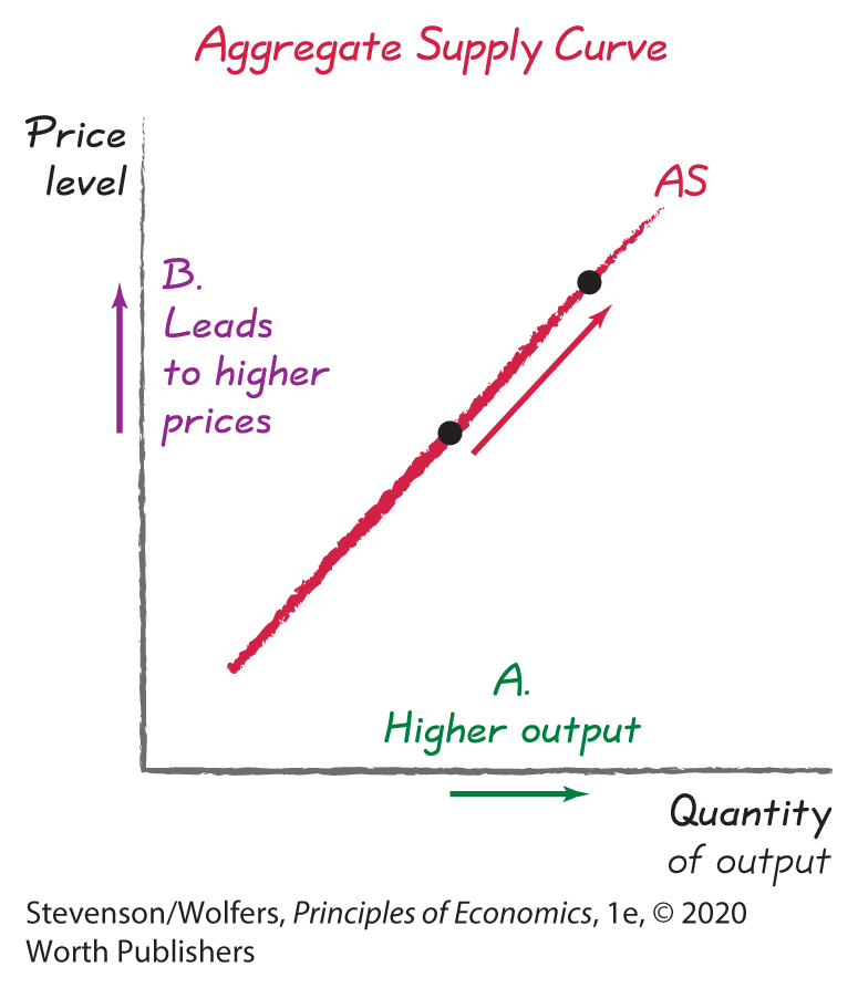
A strong economy with high GDP is good news for Outback Steakhouse because when incomes are high, your customers are more willing to splurge on a steak dinner. When the economy is doing particularly well, you’ll find your restaurants overflowing with customers, and you’ll need to pay your staff overtime to keep up. Even then, you might not be able to keep up, and some of your customers might leave rather than wait two hours for a table.

A strong economy can lead to excess demand given your limited seating capacity. In the long run, if business continues to boom, it’s worth building more restaurants. But that takes years; in the short run, you’re stuck with your existing seating capacity, which means it’s time to raise your prices. After all, even with higher prices, you can still fill your restaurant. And those higher prices will help cover your overtime bill.

The aggregate supply curve describes what happens, on average, across the millions of businesses that make up the U.S. economy. Outback’s story is relevant, because when GDP is high, millions of businesses are in a similar situation to Outback Steakhouse. Many of these businesses will respond to their excess demand much as Outback did, by raising their prices a bit. The result is that in periods of high GDP, the average price level will be a bit higher than it would otherwise be.

Lower output leads to lower prices.

The graph plots quantity of output against price level. The horizontal axis shows a rightward arrow and accompanying text that reads, A, Lower output. The vertical axis shows an upward arrow and the accompanying text that reads, B, Leads to lower prices. The upward-sloping aggregate supply curve is labeled A S and has two distinct points. An upward arrow points from the lower point to the higher point on the curve.

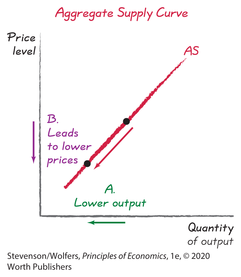
On the other hand, a weaker economy will typically lead to lower prices. To see why, let’s return to the dark days of 2009, when the economy was so weak that few people had extra cash to spend on restaurant meals. It took a toll on Outback Steakhouse, which reported that it “experienced declining revenues … and incurred operating losses.” Such losses reflect the reality that half-empty restaurants are rarely profitable.

Outback was facing a problem of insufficient demand, as the quantity of restaurant meals demanded at the prevailing price was far below the quantity that Outback wished to supply. In response, Outback offered lower prices. CEO Jeff Smith rolled out a new menu that featured “prices that are easy on the wallet,” including 15 meals under $15, and some as low as $9.95. He says that decision was one of his most difficult moments as a manager, but ultimately one of his most important successes. Because Outback’s staff barely had enough customers to stay busy, the marginal cost of serving extra meals was particularly low.

Lower GDP leads to lower prices.

When GDP is low, millions of businesses face insufficient demand. Like Outback, most will find that their marginal costs are low when they’re producing well below their capacity. They’ll follow the same logic as Jeff Smith and respond to insufficient demand with lower prices. The result is that in periods of low GDP, the average price level across the whole economy will tend to be a bit lower than it would otherwise be.

The aggregate supply curve is upward-sloping because higher output leads to a higher price level.

The figures in the margin show that lower output levels are associated with a lower average price level and higher output levels are associated with a higher average price level. Put the pieces together, and you’ve constructed the upward sloping aggregate supply curve.

Analyzing Aggregate Supply

You’ll find the aggregate supply curve to be helpful because you can use it to forecast how changing market conditions will affect economic conditions. As you do so, make sure to distinguish between a change in the price level (or a change in output), which causes a movement along the aggregate supply curve, from shifts in other factors that cause the price level to change at a given level of output, leading the aggregate supply curve to shift.

Changes in the price level lead to movements along the aggregate supply curve.

The aggregate supply curve illustrates how different price levels are associated with suppliers producing different levels of output. You can use it to assess how the price level will respond to changes in output or how output will respond to changes in the price level. The green arrow in Figure 5 illustrates how a movement along the aggregate supply curve to a higher price level is also associated with suppliers producing a higher quantity of output. (Alternatively phrased, it shows that higher output leads suppliers to push the price level higher.) The purple arrow shows that a lower price level leads to a movement along the aggregate supply curve, but this time to producing a lower quantity of output. (Or to say it the other way, it shows that lower output leads suppliers to nudge the price level lower.)

Figure 5 | The Aggregate Supply Curve

The graph plots quantity of output against price level and depicts an upward-sloping aggregate supply curve with three distinct points on it. An upward arrows points from the point in the centre of the curve to the point above and the accompanying text reads higher output means more producers have excess demand and higher marginal costs, leading more of them to charge higher prices. A downward arrow extends along the point in the centre of the curve to the point below and the accompanying text reads, Lower output means more producers have excess capacity and lower marginal costs, leading more of them to charge lower prices.

What causes the aggregate supply curve to shift? I’m glad you asked …

Changes in production costs shift the aggregate supply curve.

The costs of production are central to pricing decisions. And that matters because changing production costs cause suppliers to change the prices they’ll charge at any given level of output, thereby causing the aggregate supply curve to shift.

Lower production costs lead businesses to charge lower prices. As a result, lower production costs reduce the average price level across the whole economy (at any given level of output), thereby shifting the aggregate supply curve downward or to the right. Because this shift leads to an increase in the quantity of output associated with any given price, we say that lower production costs lead to an increase in aggregate supply. This increase arises because lower production costs boost the profitability of producing stuff, leading suppliers to increase the quantity of output they’ll produce at any given price level. Panel A on the left of Figure 6 shows that an increase in aggregate supply—by shifting the aggregate supply curve to the right—leads to both higher GDP and a lower price level. That is, it causes an economic expansion accompanied by deflation. (In reality there are often other factors driving inflation, and so this might lead to a decrease in inflation rather than outright deflation.)

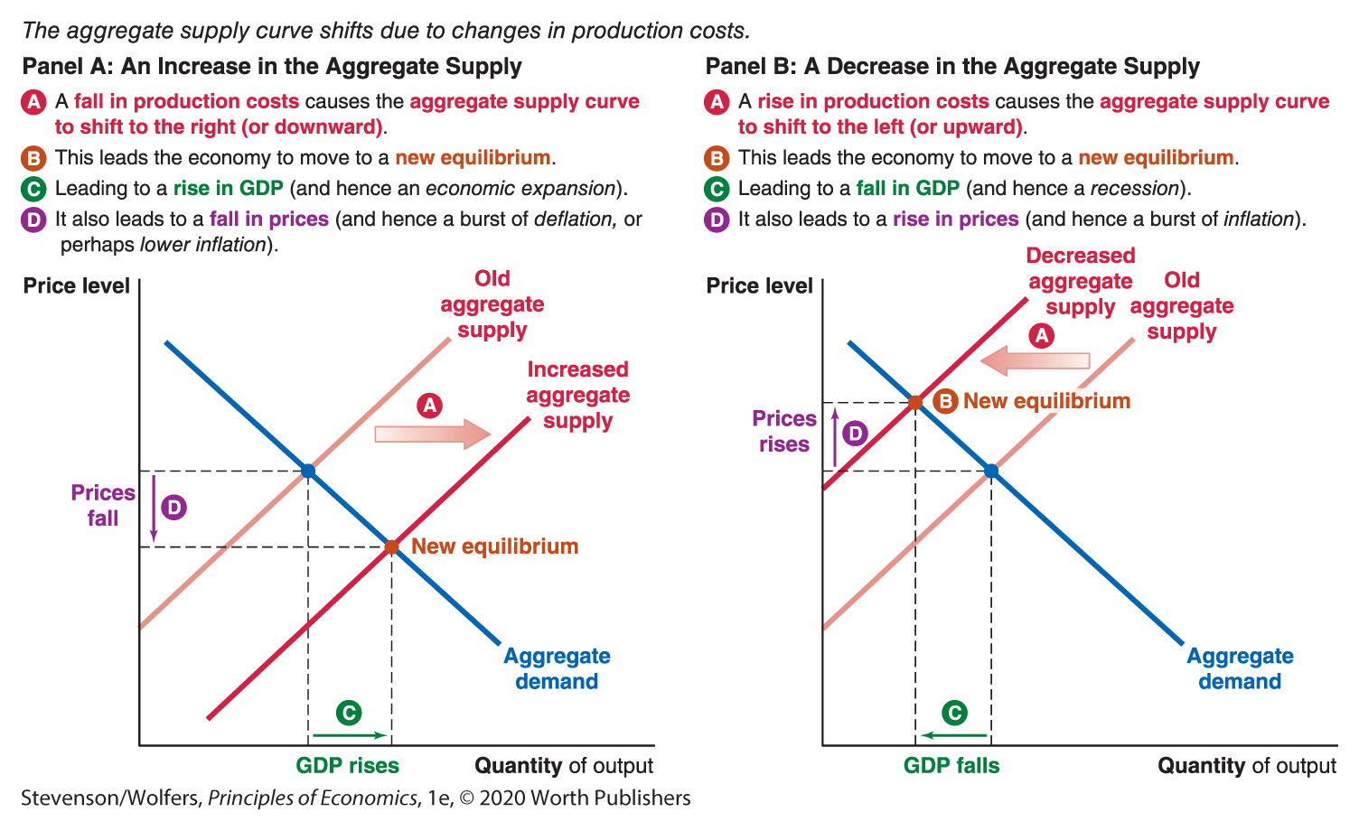
Figure 6 | Shifts in Aggregate Supply

The introductory text reads as follows:

The first graph plots quantity of output against price level and depicts a downward-sloping curve and two upward-sloping, parallel curves. The old aggregate supply curve is higher than the increased aggregate supply curve and intersects the aggregate demand curve at a point on the upper segment of the aggregate demand curve. The increased aggregate supply curve intersects the aggregate demand curve at a point on the lower segment of the curve labeled new equilibrium. Dashed lines extend from these points of intersection to meet the horizontal and vertical axis. The rise in G D P is denoted by the gap between the points on the horizontal axis and the fall in prices is denoted by the gap between the points on the vertical axis. The shift of the increased aggregate supply curve to the right is denoted by an arrow labeled A.

The aggregate supply curve shifts due to changes in production costs.

Panel A: An Increase in the Aggregate Supply

A, A fall in production costs causes the aggregate supply curve to shift to the right (or downward).

B, This leads the economy to move to a new equilibrium.

C, Leading to a rise in G D P (and hence an economic expansion).

D, It also leads to a fall in prices (and hence a burst of deflation, or perhaps lower inflation).

The introductory text to the second graph reads as follows:

Panel B: A Decrease in the Aggregate Supply

A rise in production costs causes the aggregate supply curve to shift to the left (or upward).

This leads the economy to move to a new equilibrium.

Leading to a fall in G D P (and hence a recession).

It also leads to a rise in prices (and hence a burst of inflation).

The second graph plots quantity of output against price level and shows a downward-sloping curve and two upward-sloping, parallel curves. The decreased aggregate supply curve is higher than the increased aggregate supply curve and intersects the aggregate demand curve at a point labeled B, which also denotes the new equilibrium, on the upper segment of the aggregate demand curve. The old aggregate supply curve intersects the aggregate demand curve at a point on the lower segment of the curve labeled new equilibrium. Dashed lines extend from these points of intersection to meet the horizontal and vertical axis. The fall in G D P is denoted by the gap between the points on the horizontal axis and is labeled C. The rise in prices is denoted by the gap between the points on the vertical axis. The shift of the decreased aggregate supply curve to the left is denoted by an arrow labeled A.

By contrast, higher production costs lead businesses to charge higher prices. The resulting rise in the average price level (at any given level of output) shifts the aggregate supply curve upward or to the left. Because this decreases the quantity of output associated with any given price, we say that higher production costs lead to a decrease in aggregate supply. Panel B on the right of Figure 6 shows that a decrease in aggregate supply—by shifting the aggregate supply curve to the left—leads to both lower GDP and a higher price level. This combination of declining GDP (and hence economic stagnation) and rising prices (and hence inflation) is sometimes called stagflation.

Aggregate supply shifts in response to changes in production costs, which can be caused by shifts in:

1. Input prices
2. Productivity
3. The exchange rate

An aside: We usually describe curves shifting left or right, rather than up or down. But sometimes you might find it more intuitive to think about the aggregate supply curve as shifting up rather than left when higher production costs lead businesses to raise prices. Both descriptions are accurate. Likewise, it’s just as accurate to say that lower production costs shift the aggregate supply curve down as it is to say they’ll shift the curve to the right. What’s important is that you shift your way to the right answer.

Shifts in Aggregate Supply

There are three key factors that shift production costs and hence the aggregate supply curve: shifts in input prices, productivity, and the exchange rate. Let’s explore each in turn.

Supply shifter one: Higher input prices raise production costs.

Higher energy prices make everything more expensive.

The interdependence principle emphasizes the importance of linkages between markets, and it’s especially relevant to understanding how geopolitical tensions in the Middle East can play a central role in the pricing decisions of many suppliers, including the Outback Steakhouse. Those tensions led to cutbacks in oil production that pushed up oil prices, setting off a chain reaction. Initially, products made from oil—like gasoline, heating oil, and propane—become more expensive. In turn, those higher costs made it more expensive to operate a restaurant as they raised the costs of running a commercial kitchen, heating a restaurant, and trucking ingredients across the country. Eventually, these higher marginal costs forced Outback Steakhouse to raise its prices.

The graph plots quantity of output against price level and shows three upward-sloping, parallel A S curves. Arrows depict that the A S curve shifts above for higher input prices whereas it shifts below for lower input prices.

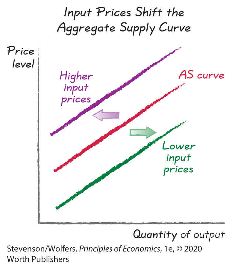
A similar story played out across many sectors of the economy, as businesses discovered that higher oil prices led to higher prices for a range of inputs that were produced using oil—including plastics, fertilizers, and rubber. Just as higher marginal costs led Outback Steakhouse to raise its prices, millions of other businesses raised their prices when their marginal costs rose. And so the average price level set by suppliers at a given level of output rose, which led to a decrease in aggregate supply.

This oil shock is a specific example of a more general phenomenon: Any time the price of your inputs rises, so will your marginal costs, and higher marginal costs lead producers to set higher prices, which shifts the aggregate supply curve to the left (or up). Indeed, labor is one of Outback’s most important inputs (as it is for many businesses), which means that sharp wage changes can cause the aggregate supply curve to shift. A few years ago executives at Outback Steakhouse reported that higher wages “have increased our labor costs in the last three years,” and in response they had addressed “increased costs by increasing menu prices.”

Supply shifter two: Weaker productivity raises production costs.

The graph plots quantity of output against price level and shows three upward-sloping, parallel A S curves. Arrows depict that the A S curve shifts above for lower productivity whereas it shifts below for higher productivity.

Your company’s productivity also changes your production costs, as a less productive company needs to buy more of each input to produce the same output. Because productivity determines marginal costs, it also impacts the prices businesses charge at any given level of GDP. For example, productivity growth slowed quite dramatically in the mid-1970s, and many businesses found their production costs to be higher than they had expected them to be. Those higher costs led businesses to raise their prices. The result was a decrease in aggregate supply, shifting the curve to the left (or upward). It also works the other way, and more rapid productivity growth increases aggregate supply, thereby shifting the aggregate supply curve to the right (or downward).

Supply shifter three: A depreciating U.S. dollar raises production costs and reduces competition from overseas.

Changes in the nominal exchange rate also shift pricing decisions and hence aggregate supply. Remember, the exchange rate is the price of a U.S. dollar in another currency. For instance, when the exchange rate is 120 Japanese yen per dollar, that means that one U.S. dollar costs 120 Japanese yen. We say that the U.S. dollar depreciates when the price of a U.S. dollar falls, say to 100 yen. This means the U.S. dollar becomes cheaper for foreigners to buy, but it also means that foreign currency is more expensive for Americans to buy because it’ll cost more dollars to buy a specific quantity of yen.

This really matters for businesses that rely on imported inputs because a depreciating U.S. dollar raises the cost of their imported inputs. For example, when an Outback Steakhouse offers Wagyu beef imported from Japan, a depreciating U.S. dollar means that it will cost Outback more dollars to import the same quantity of Japanese beef. These higher marginal costs lead Outback’s executives to raise their prices.

The graph plots quantity of output against price level and shows three upward-sloping, parallel A S curves. Arrows depict that the A S curve shifts above when the U S dollar depreciates and it shifts below when U S dollar appreciates.

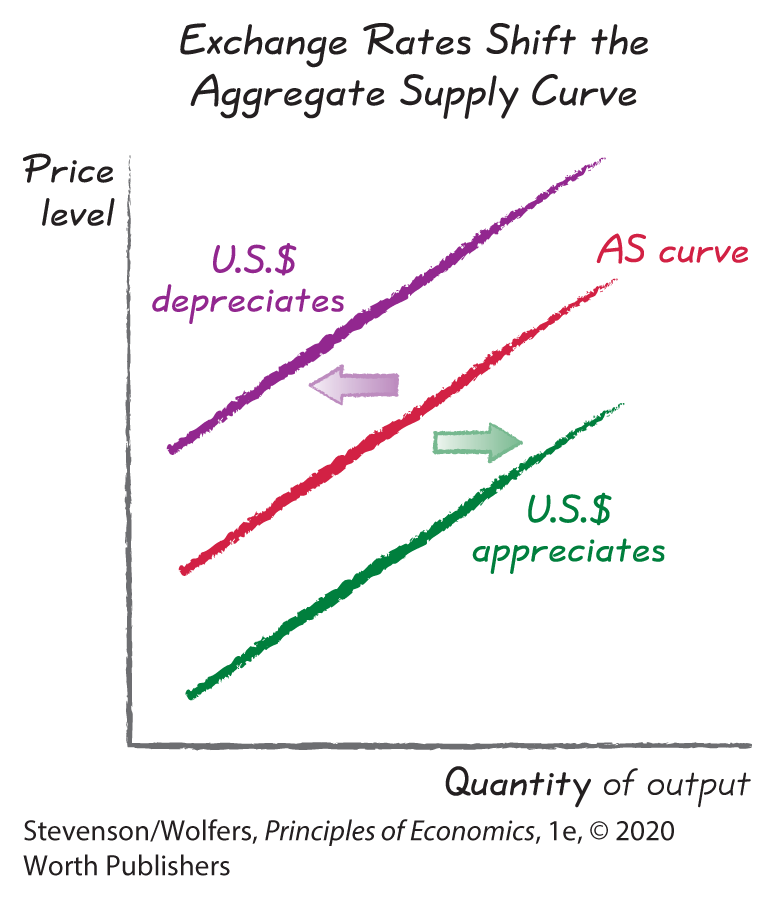
The exchange rate also matters to businesses such as Ford or General Motors that compete with imported products because a depreciating U.S. dollar raises the price (in dollars) of goods made by foreign competitors like Toyota. This weaker competitive pressure might lead domestic producers to raise their prices. Alternatively, if your business exports its output, a depreciating U.S. dollar makes your foreign customers willing to pay more (in dollars) for your products. This increased pressure from foreign customers will lead many American exporters to raise the prices they charge their American customers.

Consequently, a depreciation in the U.S. dollar leads suppliers to set higher prices at any level of output, leading to a decrease in aggregate supply. By contrast, an appreciation of the dollar leads suppliers to set lower prices at any level of output, leading to an increase in aggregate supply.

Interpreting the DATA

How a trade war shifted the aggregate supply curve

A shock to aggregate demand, or aggregate supply?

When President Trump imposed tariffs—effectively an additional sales tax—on imported goods, many proponents of the policy focused on the effects on aggregate demand. They hoped that these tariffs would lead to fewer imports, and hence boost net exports (which are exports less imports) and thus aggregate demand. What they didn’t count on was that China and Europe would retaliate with their own tariffs, designed to reduce American exports in roughly equal measure. When lower imports are matched by lower exports, there’s no effect on net exports nor on aggregate demand.

The graph plots quantity of output against price level and shows upward-sloping parallel supply curves. An arrow denotes that the A S curve shifts above for higher tariffs.

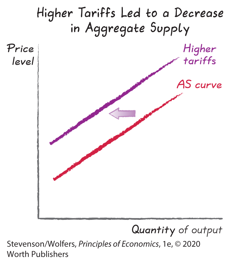
But these tariffs had a more important effect on aggregate supply. More than half of all imports to the United States are used as inputs by American businesses in the production of their goods and services. Tariffs raised the cost of purchasing these foreign inputs.

This constituted a major rise in input costs for sellers who were particularly reliant on foreign goods. For example, Jeff Starin, president of Rostar Filters, now faces hundreds of thousands of dollars in tariffs on automotive filters he imports from China. He doesn’t see a better alternative than continuing to import filters because finding alternative sources also involves higher costs. He decided to pass those higher costs on to his customers. The bottom line according to Starin is that for “the owner of a vehicle, their brake job just went up by $120.” Many other businesses have also said that increased tariffs mean they must increase prices for consumers. All this means that the aggregate supply curve shifted up (or left). And so a policy intended to increase aggregate demand ultimately instead decreased aggregate supply.

Recap: Anything that shifts production costs shifts the AS curve.

The point of this analysis isn’t to memorize a long list of factors that might shift the aggregate supply curve. Rather, focus on the bigger picture, which is that the aggregate supply curve shifts in response to changes in production costs, and we’ve identified three key shifters: input prices, productivity, and the exchange rate.

We’re now going to explore how the tools of macroeconomic policy fit in all of this. And that’s going to require a brief visit into one of the most hair-raising periods in modern economic history: the global financial crisis.