Now that we’ve covered the basics of creating a matrix, we’ll look at some common operations performed with matrices. These include performing linear algebra operations, matrix indexing, and matrix filtering.
You can perform various linear algebra operations on matrices, such as matrix multiplication, matrix scalar multiplication, and matrix addition. Using y from the preceding example, here is how to perform those three operations:
> y %*% y  # mathematical matrix multiplication
  [,1] [,2]
[1,] 7   15
[2,]10   22
> 3*y  # mathematical multiplication of matrix by scalar
  [,1] [,2]
[1,] 3    9
[2,] 6   12
> y+y  # mathematical matrix addition
  [,1] [,2]
[1,] 2    6
[2,] 4    8
For more on linear algebra operations on matrices, see Section 8.4.
The same operations we discussed for vectors in Section 2.4.2 apply to matrices as well. Here’s an example:
> z
  [,1] [,2] [,3]
[1,] 1    1    1
[2,] 2    1    0
[3,] 3    0    1
[4,] 4    0    0
> z[,2:3]
  [,1] [,2]
[1,] 1    1
[2,] 1    0
[3,] 0    1
[4,] 0    0
Here, we requested the submatrix of z consisting of all elements with column numbers 2 and 3 and any row number. This extracts the second and third columns.
Here’s an example of extracting rows instead of columns:
> y
  [,1] [,2]
[1,]11   12
[2,]21   22
[3,]31   32
> y[2:3,]
  [,1] [,2]
[1,]21   22
[2,]31   32
> y[2:3,2]
[1] 22 32
You can also assign values to submatrices:
> y
     [,1] [,2]
[1,]    1    4
[2,]    2    5
[3,]    3    6
> y[c(1,3),] <- matrix(c(1,1,8,12),nrow=2)
> y
     [,1] [,2]
[1,]    1    8
[2,]    2    5
[3,]    1   12
Here, we assigned new values to the first and third rows of y.
And here’s another example of assignment to submatrices:
> x <- matrix(nrow=3,ncol=3)
> y <- matrix(c(4,5,2,3),nrow=2)
> y
     [,1] [,2]
[1,]    4    2
[2,]    5    3
> x[2:3,2:3] <- y
> x
     [,1] [,2] [,3]
[1,]   NA   NA   NA
[2,]   NA    4    2
[3,]   NA    5    3
Negative subscripts, used with vectors to exclude certain elements, work the same way with matrices:
> y
     [,1] [,2]
[1,]    1    4
[2,]    2    5
[3,]    3    6
> y[-2,]
     [,1] [,2]
[1,]    1    4
[2,]    3    6
In the second command, we requested all rows of y except the second.
Image files are inherently matrices, since the pixels are arranged in rows and columns. If we have a grayscale image, for each pixel, we store the intensity—the brightness–of the image at that pixel. So, the intensity of a pixel in, say, row 28 and column 88 of the image is stored in row 28, column 88 of the matrix. For a color image, three matrices are stored, with intensities for red, green, and blue components, but we’ll stick to grayscale here.
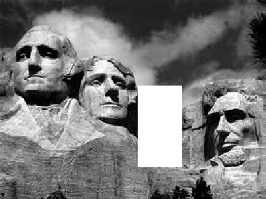
For our example, let’s consider an image of the Mount Rushmore National Memorial in the United States. Let’s read it in, using the pixmap library. (Appendix B describes how to download and install libraries.)
> library(pixmap)
> mtrush1 <- read.pnm("mtrush1.pgm")
> mtrush1
Pixmap image
  Type          : pixmapGrey
  Size          : 194×259
  Resolution    : 1×1
  Bounding box  : 0 0 259 194
> plot(mtrush1)
We read in the file named mtrush1.pgm, returning an object of class pixmap. We then plot it, as seen in Figure 3-1.

Now, let’s see what this class consists of:
> str(mtrush1)
Formal class 'pixmapGrey' [package "pixmap"] with 6 slots
  ..@ grey    : num [1:194, 1:259] 0.278 0.263 0.239 0.212 0.192 ...
  ..@ channels: chr "grey"
  ..@ size    : int [1:2] 194 259
...
The class here is of the S4 type, whose components are designated by @, rather than $. S3 and S4 classes will be discussed in Chapter 9, but the key item here is the intensity matrix, mtrush1@grey. In the example, this matrix has 194 rows and 259 columns.
The intensities in this class are stored as numbers ranging from 0.0 (black) to 1.0 (white), with intermediate values literally being shades of gray. For instance, the pixel at row 28, column 88 is pretty bright.
> mtrush1@grey[28,88]
[1] 0.7960784
To demonstrate matrix operations, let’s blot out President Roosevelt. (Sorry, Teddy, nothing personal.) To determine the relevant rows and columns, you can use R’s locator() function. When you call this function, it waits for the user to click a point within a graph and returns the exact coordinates of that point. In this manner, I found that Roosevelt’s portion of the picture is in rows 84 through 163 and columns 135 through 177. (Note that row numbers in pixmap objects increase from the top of the picture to the bottom, the opposite of the numbering used by locator().) So, to blot out that part of the image, we set all the pixels in that range to 1.0.
> mtrush2 <- mtrush1
> mtrush2@grey[84:163,135:177] <- 1
> plot(mtrush2)
The result is shown in Figure 3-2.
What if we merely wanted to disguise President Roosevelt’s identity? We could do this by adding random noise to the picture. Here’s code to do that:
# adds random noise to img, at the range rows,cols of img; img and the
# return value are both objects of class pixmap; the parameter q
# controls the weight of the noise, with the result being 1-q times the
# original image plus q times the random noise
blurpart <- function(img,rows,cols,q) {
  lrows <- length(rows)
  lcols <- length(cols)
  newimg <- img
  randomnoise <- matrix(nrow=lrows, ncol=ncols,runif(lrows*lcols))
  newimg@grey <- (1-q) * img@grey + q * randomnoise
  return(newimg)
}
As the comments indicate, we generate random noise and then take a weighted average of the target pixels and the noise. The parameter q controls the weight of the noise, with larger q values producing more blurring. The random noise itself is a sample from U(0,1), the uniform distribution on the interval (0,1). Note that the following is a matrix operation:
newimg@grey <- (1-q) * img@grey + q * randomnoise
So, let’s give it a try:
> mtrush3 <- blurpart(mtrush1,84:163,135:177,0.65)
> plot(mtrush3)
The result is shown in Figure 3-3.

Filtering can be done with matrices, just as with vectors. You must be careful with the syntax, though. Let’s start with a simple example:
> x
     x
[1,] 1 2
[2,] 2 3
[3,] 3 4
> x[x[,2] >= 3,]
     x
[1,] 2 3
[2,] 3 4
Again, let’s dissect this, just as we did when we first looked at filtering in Chapter 2:
> j <- x[,2] >= 3
> j
[1] FALSE  TRUE  TRUE
Here, we look at the vector x[,2], which is the second column of x, and determine which of its elements are greater than or equal to 3. The result, assigned to j, is a Boolean vector.
Now, use j in x:
> x[j,]
     x
[1,] 2 3
[2,] 3 4
Here, we compute x[j,]—that is, the rows of x specified by the true elements of j—getting the rows corresponding to the elements in column 2 that were at least equal to 3. Hence, the behavior shown earlier when this example was introduced:
> x
     x
[1,] 1 2
[2,] 2 3
[3,] 3 4
> x[x[,2] >= 3,]
     x
[1,] 2 3
[2,] 3 4
For performance purposes, it’s worth noting again that the computation of j here is a completely vectorized operation, since all of the following are true:
The object
x[,2]is a vector.The operator
>=compares two vectors.The number 3 was recycled to a vector of 3s.
Also note that even though j was defined in terms of x and then was used to extract from x, it did not need to be that way. The filtering criterion can be based on a variable separate from the one to which the filtering will be applied. Here’s an example with the same x as above:
> z <- c(5,12,13)
> x[z %% 2 == 1,]
     [,1] [,2]
[1,]    1    4
[2,]    3    6
Here, the expression z %% 2 == 1 tests each element of z for being an odd number, thus yielding (TRUE,FALSE,TRUE). As a result, we extracted the first and third rows of x.
Here is another example:
> m
     [,1] [,2]
[1,]    1    4
[2,]    2    5
[3,]    3    6
> m[m[,1] > 1 & m[,2] > 5,]
[1] 3 6
We’re using the same principle here, but with a slightly more complex set of conditions for row extraction. (Column extraction, or more generally, extraction of any submatrix, is similar.) First, the expression m[,1] > 1 compares each element of the first column of m to 1 and returns (FALSE,TRUE,TRUE). The second expression, m[,2] > 5, similarly returns (FALSE,FALSE,TRUE). We then take the logical AND of (FALSE,TRUE,TRUE) and (FALSE,FALSE,TRUE), yielding (FALSE,FALSE,TRUE). Using the latter in the row indices of m, we get the third row of m.
Note that we needed to use &, the vector Boolean AND operator, rather than the scalar one that we would use in an if statement, &&. A complete list of such operators is given in Section 7.2.
The alert reader may have noticed an anomaly in the preceding example. Our filtering should have given us a submatrix of size 1 by 2, but instead it gave us a two-element vector. The elements were correct, but the data type was not. This would cause trouble if we were to then input it to some other matrix function. The solution is to use the drop argument, which tells R to retain the two-dimensional nature of our data. We’ll discuss drop in detail in Section 3.6 when we examine unintended dimension reduction.
Since matrices are vectors, you can also apply vector operations to them. Here’s an example:
> m
     [,1] [,2]
[1,]    5   −1
[2,]    2   10
[3,]    9   11
> which(m > 2)
[1] 1 3 5 6
R informed us here that, from a vector-indexing point of view, elements 1, 3, 5, and 6 of m are larger than 2. For example, element 5 is the element in row 2, column 2 of m, which we see has the value 10, which is indeed greater than 2.
This example demonstrates R’s row() and col() functions, whose arguments are matrices. For example, for a matrix a, row(a[2,8]) will return the row number of that element of a, which is 2. Well, we knew row(a[2,8]) is in row 2, didn’t we? So why would this function be useful?
Let’s consider an example. When writing simulation code for multivariate normal distributions—for instance, using mvrnorm() from the MASS library—we need to specify a covariance matrix. The key point for our purposes here is that the matrix is symmetric; for example, the element in row 1, column 2 is equal to the element in row 2, column 1.
Suppose that we are working with an n-variate normal distribution. Our matrix will have n rows and n columns, and we wish each of the n variables to have variance 1, with correlation rho between pairs of variables. For n = 3 and rho = 0.2, for example, the desired matrix is as follows:
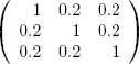
Here is code to generate this kind of matrix:
1    makecov <- function(rho,n) {
2       m <- matrix(nrow=n,ncol=n)
3       m <- ifelse(row(m) == col(m),1,rho)
4       return(m)
5    }
Let’s see how this works. First, as you probably guessed, col() returns the column number of its argument, just as row() does for the row number. Then the expression row(m) in line 3 returns a matrix of integer values, each one showing the row number of the corresponding element of m. For instance,
> z
     [,1] [,2]
[1,]    3    6
[2,]    4    7
[3,]    5    8
> row(z)
     [,1] [,2]
[1,]    1    1
[2,]    2    2
[3,]    3    3
Thus the expression row(m) == col(m) in the same line returns a matrix of TRUE and FALSE values, TRUE values on the diagonal of the matrix and FALSE values elsewhere. Once again, keep in mind that binary operators—in this case, ==—are functions. Of course, row() and col() are functions too, so this expression:
row(m) == col(m)
applies that function to each element of the matrix m, and it returns a TRUE/FALSE matrix of the same size as m. The ifelse() expression is another function call.
ifelse(row(m) == col(m),1,rho)
In this case, with the argument being the TRUE/FALSE matrix just discussed, the result is to place the values 1 and rho in the proper places in our output matrix.