Two functions are handy for applying functions to lists: lapply and sapply.
The function lapply() (for list apply) works like the matrix apply() function, calling the specified function on each component of a list (or vector coerced to a list) and returning another list. Here’s an example:
> lapply(list(1:3,25:29),median)
[[1]]
[1] 2

[[2]]
[1] 27
R applied median() to 1:3 and to 25:29, returning a list consisting of 2 and 27.
In some cases, such as the example here, the list returned by lapply() could be simplified to a vector or matrix. This is exactly what sapply() (for simplified [l]apply) does.
> sapply(list(1:3,25:29),median)
[1]  2 27
You saw an example of matrix output in Section 2.6.2. There, we applied a vectorized, vector-valued function—a function whose return value is a vector, each of whose components is vectorized— to a vector input. Using sapply(), rather than applying the function directly, gave us the desired matrix form in the output.
The text concordance creator, findwords(), which we developed in Section 4.2.4, returns a list of word locations, indexed by word. It would be nice to be able to sort this list in various ways.
Recall that for the input file testconcorda.txt, we got this output:
$the
[1]  1  5 63

$here
[1] 2

$means
[1] 3

$that
[1]  4 40
...
Here’s code to present the list in alphabetical order by word:
1    # sorts wrdlst, the output of findwords() alphabetically by word
2    alphawl <- function(wrdlst) {
3       nms <- names(wrdlst) # the words
4       sn <- sort(nms)  # same words in alpha order
5       return(wrdlst[sn])  # return rearranged version
6    }
Since our words are the names of the list components, we can extract the words by simply calling names(). We sort these alphabetically, and then in line 5, we use the sorted version as input to list indexing, giving us a sorted version of the list. Note the use of single brackets, rather than double, as the former are required for subsetting lists. (You might also consider using order() instead of sort(), which we’ll look at in Section 8.3.)
Let’s try it out.
> alphawl(wl)
$and
[1] 25

$be
[1] 67

$but
[1] 32

$case
[1] 17

$consists
[1] 20 41

$example
[1] 50
...
It works fine. The entry for and was displayed first, then be, and so on.
We can sort by word frequency in a similar manner.
1    # orders the output of findwords() by word frequency
2    freqwl <- function(wrdlst) {
3       freqs <- sapply(wrdlst,length)  # get word frequencies
4       return(wrdlst[order(freqs)])
5    }
In line 3, we are using the fact that each element in wrdlst is a vector of numbers representing the positions in our input file at which the given word is found. Calling length() on that vector gives us the number of times the given word appears in that file. The result of calling sapply() will be the vector of word frequencies.
We could use sort() here again, but order() is more direct. This latter function returns the indices of a sorted vector with respect to the original vector. Here’s an example:
> x <- c(12,5,13,8)
> order(x)
[1] 2 4 1 3
The output here indicates that x[2] is the smallest element in x, x[4] is the second smallest, and so on. In our case, we use order() to determine which word is least frequent, second least frequent, and so on. Plugging these indices into our word list gives us the same word list but in order of frequency.
Let’s check it.
> freqwl(wl)
$here
[1] 2

$means
[1] 3

$first
[1] 6
...

$that
[1]  4 40

$`in`
[1]  8 15

$line
[1] 10 24
...
$this
[1]  9 16 29 33

$of
[1] 11 21 42 56

$output
[1] 12 19 39 57
Yep, ordered from least to most frequent.
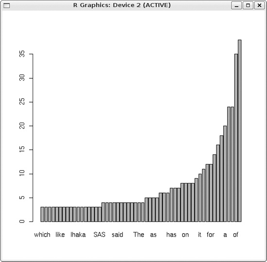
We can also do a plot of the most frequent words. I ran the following code on an article on R in the New York Times, “Data Analysts Captivated by R’s Power,” from January 6, 2009.
> nyt <- findwords("nyt.txt")
Read 1011 items
> snyt <- freqwl(nyt)
> nwords <- length(ssnyt)
> barplot(ssnyt[round(0.9*nwords):nwords])
My goal was to plot the frequencies of the top 10 percent of the words in the article. The results are shown in Figure 4-1.
Let’s use the lapply() function in our abalone gender example in Section 2.9.2. Recall that at one point in that example, we wished to know the indices of the observations that were male, female, and infant. For an easy demonstration, let’s use the same test case: a vector of genders.
g <- c("M","F","F","I","M","M","F")A more compact way of accomplishing our goal is as follows:
> lapply(c("M","F","I"),function(gender) which(g==gender))
[[1]]
[1] 1 5 6

[[2]]
[1] 2 3 7

[[3]]
[1] 4
The lapply() function expects its first argument to be a list. Here it was a vector, but lapply() will coerce that vector to a list form. Also, lapply() expects its second argument to be a function. This could be the name of a function, as you saw before, or the actual code, as we have here. This is an anonymous function, which you’ll learn more about in Section 7.13.
Then lapply() calls that anonymous function on "M", then on "F", and then on "I". In that first case, the function calculates which(g=="M"), giving us the vector of indices in g of the males. After determining the indices for the females and infants, lapply() will return the three vectors in a list.
Note that even though the object of our main attention is the vector g of genders, it is not the first argument in the lapply() call in the example. Instead, that argument is an innocuous-looking vector of the three possible gender encodings. By contrast, g is mentioned only briefly in the function, as the second actual argument. This is a common situation in R. An even better way to do this will be presented in Section 6.2.2.