Multiplying a vector by a scalar works directly, as you saw earlier. Here’s another example:
> y
[1]  1  3  4 10
> 2*y
[1]  2  6  8 20
If you wish to compute the inner product (or dot product) of two vectors, use crossprod(), like this:
> crossprod(1:3,c(5,12,13))
     [,1]
[1,]   68
The function computed 1 · 5 + 2 · 12 + 3 · 13 = 68.
Note that the name crossprod() is a misnomer, as the function does not compute the vector cross product. We’ll develop a function to compute real cross products in Section 8.4.1.
For matrix multiplication in the mathematical sense, the operator to use is %*%, not *. For instance, here we compute the matrix product:
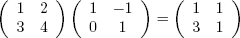
Here’s the code:
> a
     [,1] [,2]
[1,]    1    2
[2,]    3    4
> b
     [,1] [,2]
[1,]    1   −1
[2,]    0    1
> a %*% b
     [,1] [,2]
[1,]    1    1
[2,]    3    1
The function solve() will solve systems of linear equations and even find matrix inverses. For example, let’s solve this system:

Its matrix form is as follows:

Here’s the code:
> a <- matrix(c(1,1,-1,1),nrow=2,ncol=2)
> b <- c(2,4)
> solve(a,b)
[1] 3 1
> solve(a)
  [,1] [,2]
[1,]  0.5  0.5
[2,] −0.5  0.5
In that second call to solve(), the lack of a second argument signifies that we simply wish to compute the inverse of the matrix.
Here are a few other linear algebra functions:
t(): Matrix transposeqr(): QR decompositionchol(): Cholesky decompositiondet(): Determinanteigen(): Eigenvalues/eigenvectorsdiag(): Extracts the diagonal of a square matrix (useful for obtaining variances from a covariance matrix and for constructing a diagonal matrix).sweep(): Numerical analysis sweep operations
Note the versatile nature of diag(): If its argument is a matrix, it returns a vector, and vice versa. Also, if the argument is a scalar, the function returns the identity matrix of the specified size.
> m
     [,1] [,2]
[1,]    1    2
[2,]    7    8
> dm <- diag(m)
> dm
[1] 1 8
> diag(dm)
     [,1] [,2]
[1,]    1    0
[2,]    0    8
> diag(3)
     [,1] [,2] [,3]
[1,]    1    0    0
[2,]    0    1    0
[3,]    0    0    1
The sweep() function is capable of fairly complex operations. As a simple example, let’s take a 3-by-3 matrix and add 1 to row 1, 4 to row 2, and 7 to row 3.
> m
     [,1] [,2] [,3]
[1,]    1    2    3
[2,]    4    5    6
[3,]    7    8    9
> sweep(m,1,c(1,4,7),"+")
     [,1] [,2] [,3]
[1,]    2    3    4
[2,]    8    9   10
[3,]   14   15   16
The first two arguments to sweep() are like those of apply(): the array and the margin, which is 1 for rows in this case. The fourth argument is a function to be applied, and the third is an argument to that function (to the "+" function).
Let’s consider the issue of vector cross products. The definition is very simple: The cross product of vectors (x1,x2,x3) and (y1,y2,y3) in three-dimensional space is a new three-dimensional vector, as shown in Equation 8-1.

This can be expressed compactly as the expansion along the top row of the determinant, as shown in Equation 8-2.
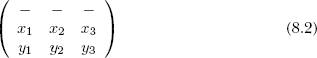
Here, the elements in the top row are merely placeholders.
Don’t worry about this bit of pseudomath. The point is that the cross product vector can be computed as a sum of subdeterminants. For instance, the first component in Equation 8-1, x2,y3 – x3y2, is easily seen to be the determinant of the submatrix obtained by deleting the first row and first column in Equation 8-2, as shown in Equation 8-3.

Our need to calculate subdeterminants—that is determinants of submatrices—fits perfectly with R, which excels at specifying submatrices. This suggests calling det() on the proper submatrices, as follows:
xprod <- function(x,y) {
   m <- rbind(rep(NA,3),x,y)
   xp <- vector(length=3)
   for (i in 1:3)
      xp[i] <- -(-1)^i * det(m[2:3,-i])
   return(xp)
}
Note that even R’s ability to specify values as NA came into play here to deal with the “placeholders” mentioned above.
All this may seem like overkill. After all, it wouldn’t have been hard to code Equation 8-1 directly, without resorting to use of submatrices and determinants. But while that may be true in the three-dimensional case, the approach shown here is quite fruitful in the n-ary case, in n-dimensional space. The cross product there is defined as an n-by-n determinant of the form shown in Equation 8-1, and thus the preceding code generalizes perfectly.
A Markov chain is a random process in which we move among various states, in a “memoryless” fashion, whose definition need not concern us here. The state could be the number of jobs in a queue, the number of items stored in inventory, and so on. We will assume the number of states to be finite.
As a simple example, consider a game in which we toss a coin repeatedly and win a dollar whenever we accumulate three consecutive heads. Our state at any time i will the number of consecutive heads we have so far, so our state can be 0, 1, or 2. (When we get three heads in a row, our state reverts to 0.)
The central interest in Markov modeling is usually the long-run state distribution, meaning the long-run proportions of the time we are in each state. In our coin-toss game, we can use the code we’ll develop here to calculate that distribution, which turns out to have us at states 0, 1, and 2 in proportions 57.1%, 28.6%, and 14.3% of the time. Note that we win our dollar if we are in state 2 and toss a head, so 0.143 × 0.5 = 0.071 of our tosses will result in wins.
Since R vector and matrix indices start at 1 rather than 0, it will be convenient to relabel our states here as 1, 2, and 3 rather than 0, 1, and 2. For example, state 3 now means that we currently have two consecutive heads.
Let pij denote the transition probability of moving from state i to state j during a time step. In the game example, for instance, p23 = 0.5, reflecting the fact that with probability 1/2, we will toss a head and thus move from having one consecutive head to two. On the other hand, if we toss a tail while we are in state 2, we go to state 1, meaning 0 consecutive heads; thus p21 = 0.5.
We are interested in calculating the vector π = (π1,...,πs), where πi is the long-run proportion of time spent at state i, over all states i. Let P denote the transition probability matrix whose ith row, jth column element is pij. Then it can be shown that π must satisfy Equation 8-4,

which is equivalent to Equation 8-5:

Here I is the identity matrix and PT denotes the transpose of P.
Any single one of the equations in the system of Equation 8-5 is redundant. We thus eliminate one of them, by removing the last row of I – P in Equation 8-5. That also means removing the last 0 in the 0 vector on the right-hand side of Equation 8-5.
But note that there is also the constraint shown in Equation 8-6.
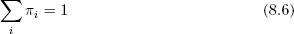
In matrix terms, this is as follows:

where 1n is a vector of n 1s.
So, in the modified version of Equation 8-5, we replace the removed row with a row of all 1s and, on the right-hand side, replace the removed 0 with a 1. We can then solve the system.
All this can be computed with R’s solve() function, as follows:
1    findpi1 <- function(p) {
2       n <- nrow(p)
3       imp <- diag(n) - t(p)
4       imp[n,] <- rep(1,n)
5       rhs <- c(rep(0,n-1),1)
6       pivec <- solve(imp,rhs)
7       return(pivec)
8 }Calculate I – PT in line 3. Note again that
diag(), when called with a scalar argument, returns the identity matrix of the size given by that argument.Replace the last row of P with 1 values in line 4.
Set up the right-hand side vector in line 5.
Solve for π in line 6.
Another approach, using more advanced knowledge, is based on eigenvalues. Note from Equation 8-4 that π is a left eigenvector of P with eigenvalue 1. This suggests using R’s eigen() function, selecting the eigenvector corresponding to that eigenvalue. (A result from mathematics, the Perron-Frobenius theorem, can be used to carefully justify this.)
Since π is a left eigenvector, the argument in the call to eigen() must be P transpose rather than P. In addition, since an eigenvector is unique only up to scalar multiplication, we must deal with two issues regarding the eigenvector returned to us by eigen():
It may have negative components. If so, we multiply by −1.
It may not satisfy Equation 8-6. We remedy this by dividing by the length of the returned vector.
Here is the code:
1    findpi2 <- function(p) {
2       n <- nrow(p)
3       # find first eigenvector of P transpose
4       pivec <- eigen(t(p))$vectors[,1]
5       # guaranteed to be real, but could be negative
6       if (pivec[1] < 0) pivec <- -pivec
7       # normalize to sum to 1
8       pivec <- pivec / sum(pivec)
9       return(pivec)
10    }
The return value of eigen() is a list. One of the list’s components is a matrix named vectors. These are the eigenvectors, with the ith column being the eigenvector corresponding to the ith eigenvalue. Thus, we take column 1 here.