Chapter 18. Neural Networks
I like nonsense; it wakes up the brain cells.
Dr. Seuss
An artificial neural network (or neural network for short) is a predictive model motivated by the way the brain operates. Think of the brain as a collection of neurons wired together. Each neuron looks at the outputs of the other neurons that feed into it, does a calculation, and then either fires (if the calculation exceeds some threshold) or doesn’t (if it doesn’t).
Accordingly, artificial neural networks consist of artificial neurons, which perform similar calculations over their inputs. Neural networks can solve a wide variety of problems like handwriting recognition and face detection, and they are used heavily in deep learning, one of the trendiest subfields of data science. However, most neural networks are “black boxes”—inspecting their details doesn’t give you much understanding of how they’re solving a problem. And large neural networks can be difficult to train. For most problems you’ll encounter as a budding data scientist, they’re probably not the right choice. Someday, when you’re trying to build an artificial intelligence to bring about the Singularity, they very well might be.
Perceptrons
Pretty much the simplest neural network is the perceptron, which approximates a single neuron with n binary inputs. It computes a weighted sum of its inputs and “fires” if that weighted sum is 0 or greater:
fromscratch.linear_algebraimportVector,dotdefstep_function(x:float)->float:return1.0ifx>=0else0.0defperceptron_output(weights:Vector,bias:float,x:Vector)->float:"""Returns 1 if the perceptron 'fires', 0 if not"""calculation=dot(weights,x)+biasreturnstep_function(calculation)
The perceptron is simply distinguishing between the half-spaces separated by the hyperplane of points x for which:
dot(weights,x)+bias==0
With properly chosen weights, perceptrons can solve a number of simple problems (Figure 18-1). For example, we can create an AND gate (which returns 1 if both its inputs are 1 but returns 0 if one of its inputs is 0) with:
and_weights=[2.,2]and_bias=-3.assertperceptron_output(and_weights,and_bias,[1,1])==1assertperceptron_output(and_weights,and_bias,[0,1])==0assertperceptron_output(and_weights,and_bias,[1,0])==0assertperceptron_output(and_weights,and_bias,[0,0])==0
If both inputs are 1, the calculation equals 2 + 2 – 3 = 1, and the output is 1. If only one of the inputs is 1, the calculation equals 2 + 0 – 3 = –1, and the output is 0. And if both of the inputs are 0, the calculation equals –3, and the output is 0.
Using similar reasoning, we could build an OR gate with:
or_weights=[2.,2]or_bias=-1.assertperceptron_output(or_weights,or_bias,[1,1])==1assertperceptron_output(or_weights,or_bias,[0,1])==1assertperceptron_output(or_weights,or_bias,[1,0])==1assertperceptron_output(or_weights,or_bias,[0,0])==0
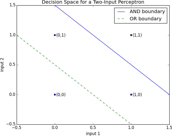
Figure 18-1. Decision space for a two-input perceptron
We could also build a NOT gate (which has one input and converts 1 to 0 and 0 to 1) with:
not_weights=[-2.]not_bias=1.assertperceptron_output(not_weights,not_bias,[0])==1assertperceptron_output(not_weights,not_bias,[1])==0
However, there are some problems that simply can’t be solved by a single perceptron. For example, no matter how hard you try, you cannot use a perceptron to build an XOR gate that outputs 1 if exactly one of its inputs is 1 and 0 otherwise. This is where we start needing more complicated neural networks.
Of course, you don’t need to approximate a neuron in order to build a logic gate:
and_gate=minor_gate=maxxor_gate=lambdax,y:0ifx==yelse1
Like real neurons, artificial neurons start getting more interesting when you start connecting them together.
Feed-Forward Neural Networks
The topology of the brain is enormously complicated, so it’s common to approximate it with an idealized feed-forward neural network that consists of discrete layers of neurons, each connected to the next. This typically entails an input layer (which receives inputs and feeds them forward unchanged), one or more “hidden layers” (each of which consists of neurons that take the outputs of the previous layer, performs some calculation, and passes the result to the next layer), and an output layer (which produces the final outputs).
Just like in the perceptron, each (noninput) neuron has a weight corresponding to each of its inputs and a bias. To make our representation simpler, we’ll add the bias to the end of our weights vector and give each neuron a bias input that always equals 1.
As with the perceptron, for each neuron we’ll sum up the products of its inputs and its weights.
But here, rather than outputting the step_function applied to that product, we’ll output a smooth approximation of it. Here we’ll use the sigmoid function (Figure 18-2):
importmathdefsigmoid(t:float)->float:return1/(1+math.exp(-t))
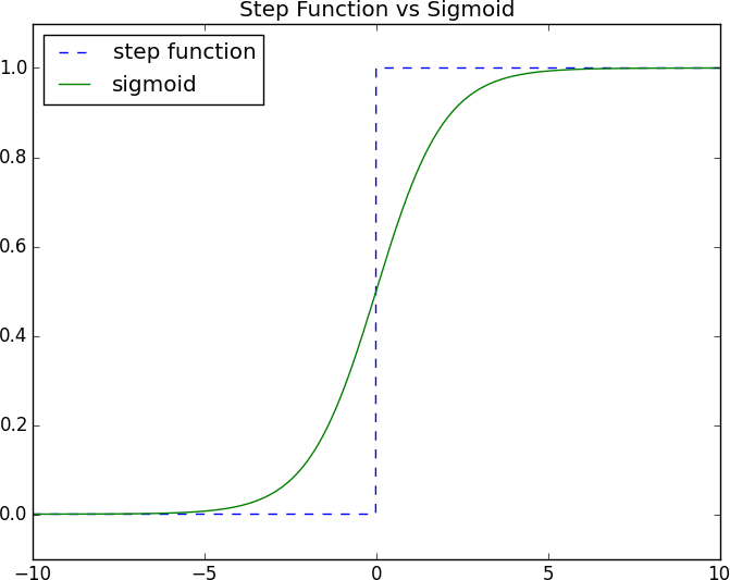
Figure 18-2. The sigmoid function
Why use sigmoid instead of the simpler step_function? In order to train a neural network, we need to use calculus, and in order to use calculus, we need smooth functions. step_function isn’t even continuous, and sigmoid is a good smooth approximation of it.
Note
You may remember sigmoid from Chapter 16, where it was called logistic. Technically “sigmoid” refers to the shape of the function and “logistic” to this particular function, although people often use the terms interchangeably.
We then calculate the output as:
defneuron_output(weights:Vector,inputs:Vector)->float:# weights includes the bias term, inputs includes a 1returnsigmoid(dot(weights,inputs))
Given this function, we can represent a neuron simply as a vector of weights whose length is one more than the number of inputs to that neuron (because of the bias weight). Then we can represent a neural network as a list of (noninput) layers, where each layer is just a list of the neurons in that layer.
That is, we’ll represent a neural network as a list (layers) of lists (neurons) of vectors (weights).
Given such a representation, using the neural network is quite simple:
fromtypingimportListdeffeed_forward(neural_network:List[List[Vector]],input_vector:Vector)->List[Vector]:"""Feeds the input vector through the neural network.Returns the outputs of all layers (not just the last one)."""outputs:List[Vector]=[]forlayerinneural_network:input_with_bias=input_vector+[1]# Add a constant.output=[neuron_output(neuron,input_with_bias)# Compute the outputforneuroninlayer]# for each neuron.outputs.append(output)# Add to results.# Then the input to the next layer is the output of this oneinput_vector=outputreturnoutputs
Now it’s easy to build the XOR gate that we couldn’t build with a single perceptron.
We just need to scale the weights up so that the neuron_outputs
are either really close to 0 or really close to 1:
xor_network=[# hidden layer[[20.,20,-30],# 'and' neuron[20.,20,-10]],# 'or' neuron# output layer[[-60.,60,-30]]]# '2nd input but not 1st input' neuron# feed_forward returns the outputs of all layers, so the [-1] gets the# final output, and the [0] gets the value out of the resulting vectorassert0.000<feed_forward(xor_network,[0,0])[-1][0]<0.001assert0.999<feed_forward(xor_network,[1,0])[-1][0]<1.000assert0.999<feed_forward(xor_network,[0,1])[-1][0]<1.000assert0.000<feed_forward(xor_network,[1,1])[-1][0]<0.001
For a given input (which is a two-dimensional vector), the hidden layer produces a two-dimensional vector consisting of the “and” of the two input values and the “or” of the two input values.
And the output layer takes a two-dimensional vector and computes “second element but not first element.” The result is a network that performs “or, but not and,” which is precisely XOR (Figure 18-3).
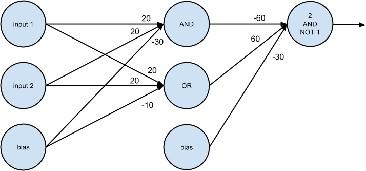
Figure 18-3. A neural network for XOR
One suggestive way of thinking about this is that the hidden layer is computing features of the input data (in this case “and” and “or”) and the output layer is combining those features in a way that generates the desired output.
Backpropagation
Usually we don’t build neural networks by hand. This is in part because we use them to solve much bigger problems—an image recognition problem might involve hundreds or thousands of neurons. And it’s in part because we usually won’t be able to “reason out” what the neurons should be.
Instead (as usual) we use data to train neural networks. The typical approach is an algorithm called backpropagation, which uses gradient descent or one of its variants.
Imagine we have a training set that consists of input vectors and corresponding target output vectors. For example, in our previous xor_network example, the input vector [1, 0] corresponded to the target output [1]. Imagine that our network has some set of weights. We then adjust the weights using the following algorithm:
-
Run
feed_forwardon an input vector to produce the outputs of all the neurons in the network. -
We know the target output, so we can compute a loss that’s the sum of the squared errors.
-
Compute the gradient of this loss as a function of the output neuron’s weights.
-
“Propagate” the gradients and errors backward to compute the gradients with respect to the hidden neurons’ weights.
-
Take a gradient descent step.
Typically we run this algorithm many times for our entire training set until the network converges.
To start with, let’s write the function to compute the gradients:
defsqerror_gradients(network:List[List[Vector]],input_vector:Vector,target_vector:Vector)->List[List[Vector]]:"""Given a neural network, an input vector, and a target vector,make a prediction and compute the gradient of the squared errorloss with respect to the neuron weights."""# forward passhidden_outputs,outputs=feed_forward(network,input_vector)# gradients with respect to output neuron pre-activation outputsoutput_deltas=[output*(1-output)*(output-target)foroutput,targetinzip(outputs,target_vector)]# gradients with respect to output neuron weightsoutput_grads=[[output_deltas[i]*hidden_outputforhidden_outputinhidden_outputs+[1]]fori,output_neuroninenumerate(network[-1])]# gradients with respect to hidden neuron pre-activation outputshidden_deltas=[hidden_output*(1-hidden_output)*dot(output_deltas,[n[i]forninnetwork[-1]])fori,hidden_outputinenumerate(hidden_outputs)]# gradients with respect to hidden neuron weightshidden_grads=[[hidden_deltas[i]*inputforinputininput_vector+[1]]fori,hidden_neuroninenumerate(network[0])]return[hidden_grads,output_grads]
The math behind the preceding calculations is not terribly difficult, but it involves some tedious calculus and careful attention to detail, so I’ll leave it as an exercise for you.
Armed with the ability to compute gradients, we can now train neural networks. Let’s try to learn the XOR network we previously designed by hand.
We’ll start by generating the training data and initializing our neural network with random weights:
importrandomrandom.seed(0)# training dataxs=[[0.,0],[0.,1],[1.,0],[1.,1]]ys=[[0.],[1.],[1.],[0.]]# start with random weightsnetwork=[# hidden layer: 2 inputs -> 2 outputs[[random.random()for_inrange(2+1)],# 1st hidden neuron[random.random()for_inrange(2+1)]],# 2nd hidden neuron# output layer: 2 inputs -> 1 output[[random.random()for_inrange(2+1)]]# 1st output neuron]
As usual, we can train it using gradient descent. One difference
from our previous examples is that here we have several parameter vectors,
each with its own gradient, which means we’ll have to call gradient_step
for each of them.
fromscratch.gradient_descentimportgradient_stepimporttqdmlearning_rate=1.0forepochintqdm.trange(20000,desc="neural net for xor"):forx,yinzip(xs,ys):gradients=sqerror_gradients(network,x,y)# Take a gradient step for each neuron in each layernetwork=[[gradient_step(neuron,grad,-learning_rate)forneuron,gradinzip(layer,layer_grad)]forlayer,layer_gradinzip(network,gradients)]# check that it learned XORassertfeed_forward(network,[0,0])[-1][0]<0.01assertfeed_forward(network,[0,1])[-1][0]>0.99assertfeed_forward(network,[1,0])[-1][0]>0.99assertfeed_forward(network,[1,1])[-1][0]<0.01
For me the resulting network has weights that look like:
[# hidden layer[[7,7,-3],# computes OR[5,5,-8]],# computes AND# output layer[[11,-12,-5]]# computes "first but not second"]
which is conceptually pretty similar to our previous bespoke network.
Example: Fizz Buzz
The VP of Engineering wants to interview technical candidates by making them solve “Fizz Buzz,” the following well-trod programming challenge:
Print the numbers 1 to 100, except that if the number is divisible
by 3, print "fizz"; if the number is divisible by 5, print "buzz";
and if the number is divisible by 15, print "fizzbuzz".
He thinks the ability to solve this demonstrates extreme programming skill. You think that this problem is so simple that a neural network could solve it.
Neural networks take vectors as inputs and produce vectors as outputs. As stated, the programming problem is to turn an integer into a string. So the first challenge is to come up with a way to recast it as a vector problem.
For the outputs it’s not tough: there are basically four classes of outputs, so we can encode the output as a vector of four 0s and 1s:
deffizz_buzz_encode(x:int)->Vector:ifx%15==0:return[0,0,0,1]elifx%5==0:return[0,0,1,0]elifx%3==0:return[0,1,0,0]else:return[1,0,0,0]assertfizz_buzz_encode(2)==[1,0,0,0]assertfizz_buzz_encode(6)==[0,1,0,0]assertfizz_buzz_encode(10)==[0,0,1,0]assertfizz_buzz_encode(30)==[0,0,0,1]
We’ll use this to generate our target vectors. The input vectors are less obvious. You don’t want to just use a one-dimensional vector containing the input number, for a couple of reasons. A single input captures an “intensity,” but the fact that 2 is twice as much as 1, and that 4 is twice as much again, doesn’t feel relevant to this problem. Additionally, with just one input the hidden layer wouldn’t be able to compute very interesting features, which means it probably wouldn’t be able to solve the problem.
It turns out that one thing that works reasonably well is to convert each number to its binary representation of 1s and 0s. (Don’t worry, this isn’t obvious—at least it wasn’t to me.)
defbinary_encode(x:int)->Vector:binary:List[float]=[]foriinrange(10):binary.append(x%2)x=x//2returnbinary# 1 2 4 8 16 32 64 128 256 512assertbinary_encode(0)==[0,0,0,0,0,0,0,0,0,0]assertbinary_encode(1)==[1,0,0,0,0,0,0,0,0,0]assertbinary_encode(10)==[0,1,0,1,0,0,0,0,0,0]assertbinary_encode(101)==[1,0,1,0,0,1,1,0,0,0]assertbinary_encode(999)==[1,1,1,0,0,1,1,1,1,1]
As the goal is to construct the outputs for the numbers 1 to 100, it would be cheating to train on those numbers. Therefore, we’ll train on the numbers 101 to 1,023 (which is the largest number we can represent with 10 binary digits):
xs=[binary_encode(n)forninrange(101,1024)]ys=[fizz_buzz_encode(n)forninrange(101,1024)]
Next, let’s create a neural network with random initial weights. It will have 10 input neurons (since we’re representing our inputs as 10-dimensional vectors) and 4 output neurons (since we’re representing our targets as 4-dimensional vectors). We’ll give it 25 hidden units, but we’ll use a variable for that so it’s easy to change:
NUM_HIDDEN=25network=[# hidden layer: 10 inputs -> NUM_HIDDEN outputs[[random.random()for_inrange(10+1)]for_inrange(NUM_HIDDEN)],# output_layer: NUM_HIDDEN inputs -> 4 outputs[[random.random()for_inrange(NUM_HIDDEN+1)]for_inrange(4)]]
That’s it. Now we’re ready to train. Because this is a more involved problem (and there are a lot more things to mess up), we’d like to closely monitor the training process. In particular, for each epoch we’ll track the sum of squared errors and print them out. We want to make sure they decrease:
fromscratch.linear_algebraimportsquared_distancelearning_rate=1.0withtqdm.trange(500)ast:forepochint:epoch_loss=0.0forx,yinzip(xs,ys):predicted=feed_forward(network,x)[-1]epoch_loss+=squared_distance(predicted,y)gradients=sqerror_gradients(network,x,y)# Take a gradient step for each neuron in each layernetwork=[[gradient_step(neuron,grad,-learning_rate)forneuron,gradinzip(layer,layer_grad)]forlayer,layer_gradinzip(network,gradients)]t.set_description(f"fizz buzz (loss: {epoch_loss:.2f})")
This will take a while to train, but eventually the loss should start to bottom out.
At last we’re ready to solve our original problem. We have one remaining issue.
Our network will produce a four-dimensional vector of numbers, but we want a single
prediction. We’ll do that by taking the argmax, which is the index of the largest value:
defargmax(xs:list)->int:"""Returns the index of the largest value"""returnmax(range(len(xs)),key=lambdai:xs[i])assertargmax([0,-1])==0# items[0] is largestassertargmax([-1,0])==1# items[1] is largestassertargmax([-1,10,5,20,-3])==3# items[3] is largest
Now we can finally solve “FizzBuzz”:
num_correct=0forninrange(1,101):x=binary_encode(n)predicted=argmax(feed_forward(network,x)[-1])actual=argmax(fizz_buzz_encode(n))labels=[str(n),"fizz","buzz","fizzbuzz"](n,labels[predicted],labels[actual])ifpredicted==actual:num_correct+=1(num_correct,"/",100)
For me the trained network gets 96/100 correct, which is well above the VP of Engineering’s hiring threshold. Faced with the evidence, he relents and changes the interview challenge to “Invert a Binary Tree.”
For Further Exploration
-
Keep reading: Chapter 19 will explore these topics in much more detail.
-
My blog post on “Fizz Buzz in Tensorflow” is pretty good.