21.1 THE FORMAL ALGEBRA OF POWER SERIES
Power series play a prominent role in much of mathematics; hence we need to know how to handle them. It is evident from the linearity of both differentiation and summation that if
then
![]()
For multiplication of two power series (we ignore for the moment the problem of the convergence of the product), write the product
![]()
How can a term in xn arise in the product? To avoid troubles, we first write the products with dummy variables of summation m and k:
We see that the condition for the term xn to arise is
m + k = n
Then, and only then, can we get a term Jtn; the sum of the exponents of the individual terms in the product must add up to the value n. Rewriting this, we get
k = n − m
Thus each coefficient wn of the product is given by corresponding finite sum of products
![]()
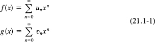
This is called the convolution of the two sequences of coefficients. Its structure is best seen in the Figure 21.1-1, where we have written on one strip the coefficients of the un series in order as you go down, and have written the coefficients of vn in the opposite order. Each coefficient wn is found from the sum of all the products when the two arrays are shifted an amount of exactly n. We have seen this before, for example in the sum of two random variables. Note that the convolution of the uk with the vm is the same as the convolution of the vm with the uk.
Figure 21.1-1 Convolution
Example 21.1-1
Consider the product exey. We get
![]()
If wn are the coefficients of the product, then the convolution gives
![]()
If (1) we write this as (multiply and divide by n!), (2) note the binomial coefficients appearing, and (3) apply the binomial expansion, we get
We have, therefore,
![]()
This is, of course, what you expect since
![]()
We have proved that the function exp x is an exponential function.
Example 21.1-2
Division of power series is done much like the division of polynomials. Using
we divide the two series:
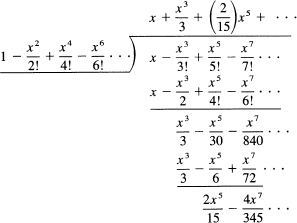
Thus, assuming that the quotient series converges, we have
We cannot expect convergence beyond the first zero of the denominator since there the quotient is infinite, and the power series, if it represented the quotient, would diverge there. We will simply state that this series does converge that far.
21.2 GENERATING FUNCTIONS
In Chapter 2 we introduced the idea of a generating function of the binomial coefficients. The expansion
![]()
is the generating function of the binomial coefficients C(n, k). We also saw that by multiplying generating functions we could find various identities. For example the equation
(1 + t)n+m = (1 + t)n(l + t)m
regarded as generating functions, leads to various identities among the binomial coefficients when we equate the corresponding linearly independent terms on both sides (the corresponding powers of t). Because the expansion of a function in a power series about a point is unique, it follows that the corresponding coefficients of like powers are equal. We can differentiate and integrate such identities to get new identities.
We now regard the expansion
![]()
as a generating function of the numbers un [or of functions of x in case un = un(x)].
Example 21.2-1
We can regard the equation
![]()
as the generating function of the numbers 1, 1, 1, …. If we differentiate this and then multiply through by t, we get
![]()
which is the generating function of the numbers 1, 2, 3, ….
Had we integrated the original expression (21.2-1) from 0 to t (and multiplied by –1), we would have found, for |t| < 1,
where in the second line we have shifted the dummy index of summation by 1. It is easy to verify that these two expansions are the same by simply writing out the first few terms and comparing the two forms.
Example 21.2-2
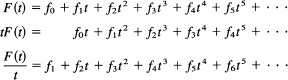
Given a probability distribution p(n) for n = 0, 1, 2,…, the corresponding generating function is
![]()
If we differentiate this expression, we get
![]()
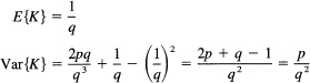
The expected value of the distribution p(k) (the mean of average) is
![]()
If we multiply the derivative Equation (21.2-5) by t and differentiate again, we get
![]()
Hence, putting t = 1, we have
![]()
Recalling that the variance is
![]()
we have that
![]()
Thus the generating function enables us to find the first and second moments of a distribution by the simple process of differentiation. Indeed, it is easy to see how to get the higher moments, if you want them, from the generating function of the distribution. The formula (21.2-8) for the variance is very useful.
A power series can, therefore, be regarded as a generating function of the coefficients. The student may notice that in this approach the convergence of the series is not important; it is the formal relationships that seem to matter. When we multiply two generating functions together, we get the corresponding generating function of the new set of numbers. We saw such a process when we multiplied two powers of (1 + t)k and compared the results. If the numbers are to be combined according to the corresponding convolution, then the corresponding coefficients of like powers are to be identified without regard to the convergence. The question of the convergence of generating functions is a delicate matter that has long been debated; it is, of course nice if the series converges, but at times useful results are obtained by the formal manipulation of generating functions without regard to the convergence or divergence of any of the expansions.
The student may wonder how we get generating functions in cases where we do not know them already. The Fibonacci numbers in the next example will show how: (1) the assumption of the generating functions of the Fibonacci numbers, (2) applying the known relationship that defines the Fibonacci numbers leads us to the generating function, and (3) the manipulation of the function to get it expanded in a formal power series, without the cost of trying to compute the general derivative, produces the coefficients.
Example 21.2-3
The Fibonacci numbers (Example 2.4-3)are defined by
![]()
we assume (1) that we have the generating function of the Fibonacci numbers:
![]()
If we multiply by t, we get
![]()
and shifting the dummy index of summation from k + 1 to k, we have
![]()
Evidently, multiplying the generating function by t lowers the index of summation by 1. This suggests that dividing by t would shift the index up by 1. We have
![]()
We are now ready to do step (2). The fundamental defining equation for the Fibonacci numbers is
![]()
We write out the three expansions in detail to see what is going on.
![]()
and the coefficients of all other powers are automatically zero because of the defining relation fn+1 – fn – fn–1 = 0. Solve for F(t) to get
![]()
or
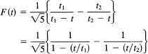
![]()
We have the generating function for the Fibonacci numbers. It is now a matter of getting it into a power series form (3). We could divide it out, but that appears to give a confusing result, so we first apply the method of partial fractions to the right-hand side.
![]()
where t1 and t2 are the roots of the quadratic in the denominator
t2 + t – 1 = 0
These roots are
![]()
After tedious algebra (and no one said that the method is easy to carry out, only that the ideas are simple), we get
![]()
A little more algebra and we have
But recalling that for this quadratic equation the product of the roots t1t2 = –1, we get
![]()
We can now divide these out using the form
![]()
to get finally for the coefficient of tn
![]()
which upon further algebra yields the value given in Example 2.4-3:
![]()
Generalization 21.2-4
From the single example of the Fibonacci numbers, we see that with any given set of numbers defined by a difference equation with constant coefficients of the form
![]()
we can do a similar process and obtain the general term in a closed form, provided we can factor the denominator into linear factors. Indeed, if quadratic factors arose, we could, at some cost in effort, divide out the quadratic factors.
1. The generating function of the sequence 1, 1, 1, … is 1/(1 – t). Show that the square of it gives the numbers 1, 2, 3, …. What does the cube give?
2. If p(n) = l/2 n+1 for n = 0, 1, 2, …, find the generating function and check that P(l) = 1. Find the mean and variance of the distribution.
3. Using the recurrence relation un = aun-1, u0 = 1, find the generating function.
4.* Using the recurrence relation un+1 = aun + bun–1 with u0 = 0, u1 = 1, find the generating function.
21.3 THE BINOMIAL EXPANSION AGAIN
In Section 2.4 we found the binomial expansion for integer n:
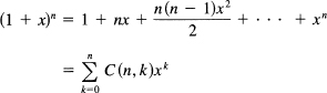
where the binomial coefficients C(n,k) are given by the formula
![]()
Looking at the expansion, we see that it is simply the Maclaurin expansion of the function (1 + x)n. We can get it directly by
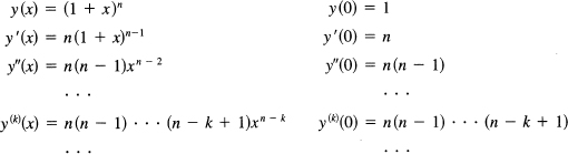
To get the coefficient of xk, the kth derivative must be diveded by k!, and we see that we get exactly the same result as we earlier found for the binomial expansion.
Now that we have two different derivations of this important result, we are in a position to compare the assumptions behind the derivations and perhaps loosen the conditions. For the earlier proof we used mathematicalinduction and were pretty well confined to positive integer exponents n. In this new derivation we are not so limited. If we believe
![]()
for the exponent n,whether or not an integer, then we have the corresponding binomial expansion. But we will now get an endless sequence of coefficients; the numerator factor will not produce a zero coefficient past some point unless n is an integer. It is natural to extend the defination of the binomial coefficients to noninteger values of n, and say
![]()
for all real values of n and integer k. (Compare with Example 9.10-3.)
We will have, for noninteger exponents n, an infinite series
![]()
What about the convergence? The ratio test gives
![]()
and as k → ∞, we see that for |x| < 1 we have convergence. We will not examine the convergence at the ends of the interval.
The student of the foundations of what we know should note that the derivative
![]()
was derived for rational numbers only, and by assumption 1 of Section 4.5 we extended it to the irrational exponents. However, if the student believes that for all real n
y = xn
is equivalent to
ln y = n ln x
then differentiating this gives
![]()
from which we get
![]()
without use of assumption 1 of Section 4.5. Thus we have an alternative derivation for the derivative of a power of x, one that may seem to make fewer assumptions.
We need to examine the binomial coefficients for negative integers. We have the definition
![]()
If we replace n by -n we get
![]()
Thus we can write (for positive n) the negative binomial coefficients as
![]()
This is the fundamental tool for converting binomial coefficients from negative exponents to positive exponents.
Example 21.3-1
Suppose we check this binomial expansion formula for posivitive exponents by observing that
![]()
We have the Maclaurin expansion for the first few terms:
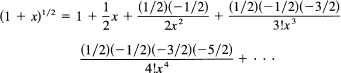
We have now to multiply this series by itself (using detached coefficients); we have
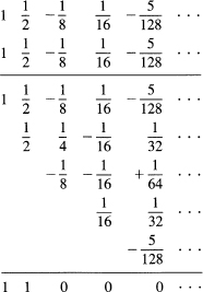
We can similarly check the binomial expansion for negative exponents by using
![]()
In this way we can find many identities among the binomial coefficients.
Example 21.3-2
First occurrence. We often want to know when something will happen for the first time. Consider the tossing of a coin, or other Bernoulli trial, with probability of success p and of failure q = 1 — p. For independent trials we have the probability of the first failure to occur on the kth trial equals: success, success, success, …, success, failure. This probability is
![]()
As a partial check of this, we examine the sum of all possible outcomes:
![]()
which is what it should be, since the first occurrence must occur sometime.
What is the expected value of this probability of first occurrence? We need the generating function of the probabilities. This generating function is (by definition)
![]()
To get the mean and variance of the distribution of first occurrence [see formula (21.2-8)], xwe need the first two derivatives of the generating function. We have
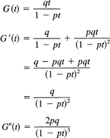
Evaluating these at t = 1, we get
Example 21.3-3
Suppose we now ask for the probability distribution of the time to the second failure (occurrence). Evidently, the first failure can occur at any time before the second, so considering all those times of first failure plus the second failure, which add up to the second failure at the kth trial, we see a convolution arising. We have a sum of all products of occurrence for the first and second failure such that the sum of their times is the given amount. The generating functions of each failure (first and second) are the same since the two are assumed to be independent. Hence, the generating function of the time to second failure is just the square of the generating function to first failure:
![]()
The individual terms involve the binomial coefficients of order —2. We have, using (21.3-3),
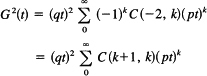
Using C(n, k) = C(n, n– k), we have
The probability distribution of the second failure is given by (k – 1)p k–2q2.
Case History 21.3-4
The Catalan numbers. The Catalan numbers occur in many different applications, but the background from which they come is, in each case, difficult to explain simply. The stages in the solution leading to them illustrate the use of many of the small ideas that we have just developed. The numbers un are defined by the convolution
![]()
or
![]()
with uo = 1. This convolution suggests immediately that we deal with generating functions. Let the generating function be
![]()
We multiply the convolution equation by tn and sum with respect to n. We see that
![]()
This can be written as a quadratic equation
![]()
whose solution is
![]()
This is no u-1 term; hence we must use the minus sign. We have, therefore,
![]()
Our problem is now to get this expression as a power series in t. To do this, we begin with the binomial expansion of the radical:
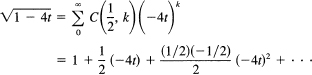
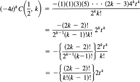
Hence
![]()
and our original expression becomes (in the second line shift the summation index)
The number un is (the coefficient of tn)
![]()
These are known as the Catalan numbers, and occur in numerous places in mathematics.
The values of the sequence of Catalan numbers can be either found one at a time from this formula, or else we can find a recurrence relation. To find a recursive formula, we write
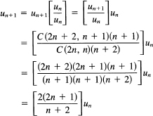
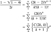
The first few Catalan numbers are uo = 1, u1 = 1, u2 = 2, u3 = 5, u4 = 14, u5 = 42, u6 = 132, u7 = 429, …. The size of the nth Catalan number can be found using Stirling’s approximation for n!
1. Write C(– 3, k) as a positive binomial coefficient.
2. Verify by expanding and multiplying out the first four powers of (1 + x)(1 + x)-1 = 1.
3. Verify by expanding and multiply ingout the fir st four terms of (1 + x) 1/2 (1 + x)–1/2 = 1.
4. Find the probability of the third occurrence at trial k.
5. Find the mean and variance of the probability distribution of the second occurrence.
6. Show that (1 + x)1/3 (1 + x)2/3 = 1 + x through the fourth-degree terms.
7. Using the Stirling approximation, find an estimate of the nth Catalan number.
21.4 EXPONENTIAL GENERATING FUNCTIONS
The form of the generating function series we assumed is the standard one. However, at times it is worth using various alternative forms. The second most common form for a generating function of the numbers un is the exponential generating function, which has the form
![]()
The difference is that we now are dealing with the original numbers un divided by nl. Note that the formulas for the mean and variance do not apply with this generating function.
Example 21.4-1
Suppose we want the moments of the normal distribution centered about the origin (for convenience). The probability density function is
![]()
and the moments are
![]()
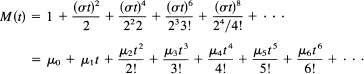
We form the exponential generating function of the moments
![]()
We have carefully arranged that inside the integral there will be the sum
Therefore, the moment generating function is of the form
![]()
The exponent from the p(x) will add to this to give us, in the exponent,
![]()
This immediately suggests completing the square:
![]()
We now have
![]()
Change the variable of integration to x – σ2t – y. This gives
![]()
This is the generating function of the moments of the normal distribution. We now express this in powers of t. We have immediately, upon expanding the exponential in a Maclaurin expansion,
It remains to equate the like powers of t. Clearly, all the odd moments are zero (the integrand is odd over a symmetric range, so this clearly checks for all the odd powers of t). For the even powers, we get
![]()
The generating function approach gives us all the moments of the normal distribution at one time.
The method just used can be applied to many situations besides finding moments of a probability distribution. With variations you can find all the integrals of a family of the form
![]()
provided you can do the corresponding integral that arises, depending on the kind of generating function you adopt. It is then a matter of expanding the generating function into powers of t and equating like terms.
1. Using a generating function, find the moments of the distribution p(x) = a exp (–ax), x ≥ 0.
2. Using a generating function, find the moments of the function sin πx, 0 ≤ x ≤ 1.
21.5 COMPLEX NUMBERS AGAIN
The expansion of the exponential function is
![]()
Suppose we make the formal substitution
x = iθ
where i = ![]() We will get
We will get
![]()
and if we rearrange this in terms of real and imaginary numbers, (using i2 = –1, i3 = –i, i4 = 1, …), we get
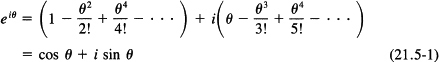
This is the famous Euler identity. The formula is sometimes written as exp (iθ) = cos θ. The formula is certainly surprising at first, so we evaluate it for a number of values.
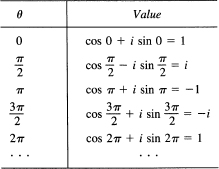
We see that each additional increase of π/2 to the angle gives a multiplicative factor of i. Thus the results are consistent with the multiplicative property of the exponential function. The particular value
eπi = –1
is very interesting as it shows that a close relationship exists between the two transcendental numbers, e and π, that dominate the calculus and its applications. (The number y = 0.577… is a very different number in the sense that it is apparently unrelated to e and π).
Let us explore the matter further and see if cos θ + i sin θ is truly an exponential. We begin with
![]()
and write each term out in the sin and cos form.
![]()
Using the addition formulas of trigonometry, we have the result
![]()
This is the de Moivre (1667–1754) identity (of whom Newton once said, “Ask Monsieur de Moivre; he knows these things better than I do.”). The identity (21.5-2) provides a very convenient way of remembering the addition formulas of trigonometry.
In this identity we can set θ = θ and use the same methods as we used in Section 3.8 for studying the exponentials, to get the fact that Euler’s and de Moivre’s identities are true for all rational powers. Using the assumption 1 of Section 4.5, they are also true for all real numbers. To get to negative exponents, we can either replace i by – i throughout, or a bit more reasonably note that
![]()
Hence cos θ – i sin θ is the reciprocal of cos θ + i sin θ.
In some respects the de Moivre identity is the heart of trigonometry;it explains
so much of what one sees. For example, it is what is behind the result (Section 2.3) where we showed that cos nx = polynomial of degree n in cos x. It is simply the nth power of the cos x + i sin x, plus noting that the real parts have only sin2 x, which is easily converted to cos2 x so the result is only in cos x.
It is possible that you might have felt better about all the formalism if we had started with
exp (ax)
and set a = i, but it would be formalism nevertheless.
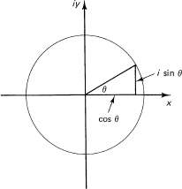
We see that |exp(ix)| = 1. If we plot cos θ + i sin θ in the complex plane (Section 5.12), we find Figure 21.5-1. This figure should give you a bit more
Figure 21.5-1 eiθ
confidence in the results obtained so far; you can see that the point described by
eiθ = cos θ + i sin θ
goes around the unit circle as θ goes from 0 to 2π, and the picture has the right periodicity for both sides of the equation. The geometric approach complements and reinforces the algebraic approach.
We write out the two Euler identities (21.5-1) (note the shift to the x variable),
eix = cos x + i sin x
e–ix = cos x – i sin x
add, and divide by 2, to get
![]()
Similarly, by subtraction we get
![]()
Thus we can convert from trigonometry to complex exponentials and back again as we please. This is useful, especially if you abbreviate eix by writing it as a new variable z:
![]()
You have
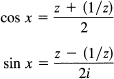
These substitutions reduce many trigonometric identities to problems in rational algebra where you do not need to recall the many trigonometric identities. In the sense of analytic geometry versus synthetic geometry, this is the analytic approach to trigonometric identities. The analytic approach to trigonometry has the corresponding power. Note that
![]()
Example 21.5-1
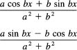
Consider the expression (compare with Section 17.4)
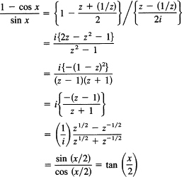
In the above derivation, we have used mainly algebra and have used trigonometry only at the two ends. Of course, the derivation is much more rapid if you know all the various identities and when to use them; the above method is useful when you have no idea of what to do with the mess of trigonometric functions. The method is especially useful in handling “regular” identities.
Example 21.5-2
Consider the Euler identity
![]()
Writing this in terms of the symbol z, we get
![]()
This is clearly a geometric progression, and we get (arranging things in a symmetric form)
which is the same as before, but a lot more directly obtained.
From the rules of exponents it follows that for complex exponents we have
exp (a + ib) = (exp a) (cos b + i sin b)
Example 21.5-3
In Example 16.5-7, we considered integrals of the form
![]()
and used integration by parts twice to get each answer. With complex exponentials we can get the two results much more easily. They are the imaginary and real parts of
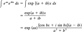
where we have ignored the constant of integration, and for the last equation have multiplied the numerator and the denominator by the complex conjugate a – ib to make the denominator real. We have now to pick out the real and imaginary parts of the right-hand side. They are
which agrees with the earlier results (a here is —a there).
What are we to think about all this formalism? Generally, most mathematicians are a lot happier when it is placed on a postulational basis of what appears to be more elementary assumptions. Engineers and scientists tend to feel that it must be true since the whole machinery works so well with the known parts of mathematics that they use daily. “Let the mathematicians make it more rigorous by the mathematician’s standards if they wish,” is their attitude, “we know it is true.”
And this illustrates much of the progress of mathematics. What was at one time assumed to be obviously true by those using it, mathematicians have later analyzed more deeply and placed on a foundation of a postulational system that is logically more satisfying to them, and the results are generally more teachable. The postulational approach makes things more compact and makes them more certain in the sense that the assumptions are fewer, more visible, and easier to study for contradictions. But the engineer’s and scientist’s view is that whatever they believe is true is up to the mathematicians to account for; and if what the mathematicians report is not what the users want, then let the mathematicians try again. Of course, what was “obvious” to the engineers has more than once turned out to be false! The rigor of mathematics is the hygiene necessary to prevent these kinds of mistakes. This process describes much of the history of mathematics. The first formalizations are often not adequate and further work must be done. Thus mathematics is a cooperative effort (with much fighting between the two sides) of creating the useful, artistic structure we call mathematics. Mathematical rigor is seldom creative, but it is a necessary criticism of intuition if we are to avoid endless mistakes. We need to take advantage of the best of both approaches.
Of course, it is often the mathematician who first notices some interesting relationship and extends, generalizes, and abstracts it before it is needed by the users of mathematics. There is both a risk and an advantage of going forward without regard to the needs of the users; you are free from petty details, but you risk making an irrelevant generalization. Much useful mathematics has thus been found, and that which is ill generalized is soon forgotten.
1. Find cos 6x in terms of powers of cos x.
Using the z notation, complete the following identities:
2. cos 2x – sin2x
3. 2 sin x cos x
4. cos3x in terms of cos x
5. tan 2x/(1 – tan2x)
6. sin x + sin 2x + sin 3x + … + sin nx
7. cos x + 2 cos 2x + 3 cos 3x + … + n cos nx
21.6 HYPERBOLIC FUNCTIONS
The Euler identities
![]()
suggest looking at the corresponding real expressions. These are the hyperbolic functions
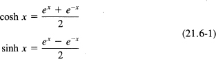
Cosh rhymes with “gosh,” and sinh is pronounced “cinch.” The other hyperbolic functions are defined similarly:
![]()
Their graphs are shown in Figure 21.6-1.
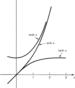
Figure 21.6-1 The hyperbolic function
Clearly, these functions are analogous to the trigonometric functions with minor differences. For example, we have
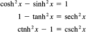
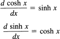
and there are no changes in sign as there are for the derivatives of the trigonometric functions.
You can show in a number of ways that the corresponding addition formulas are
![]()
For example, write out the right-hand sides as exponentials and then simplify.
The power series for the two main hyperbolic functions closely resemble those for the corresponding trigonometric functions (except that there are no changes in sign):
The inverse hyperbolic functions can be studied easily by simply interchanging the two variables and then solving for y. Thus we start with, for example,
cosh x = y
and take the inverse function
![]()
We have
![]()
This is a quadratic exp y, which is easily solved for
![]()
But since y > 0, we need to use the plus sign. Taking logs, we get
![]()
This is suitable for the range |x| > 1.
1. Write out all the definitions of the hyperbolic functions.
2. Differentiate all the hyperbolic functions.
3. Solve the quadratic that arises in finding the arctanh x. Be careful with the argument ranges.
4. Find the arcsinh x as a In function.
5. Find by differentiation the power series of cosh x and sinh x.
21.7* HYPERBOLIC FUNCTIONS CONTINUED
Why are they called “hyperbolic functions?” They are related to the hyperbola
x2 – y2 = 1
much as the trigonometric (circular) functions are related to the circle
x2 + y2 = 1
In the first equation, x = cosh θ, and in the second, x = cos 0. Correspondingly, for the y we have sinh θ and sin θ. Our problem is to identify the angle θ.
For the circular functions, we defined the angle θ as the ratio of the arc length cut out by the angle to the radius of the circle. For this analogy between the trigonometric and hyperbolic functions, we use the alternative definition of the angle as twice the area of the sector corresponding to the angle (see Figure 21.7-1). We need to find the shaded area to measure the “angle.”
The proof is made easy if we refer the hyperbola to its asymptotes. Set
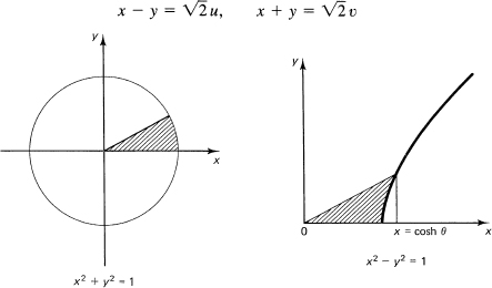
Figure 21.7-1 Hyperbolic angle
![]()
The point A has coordinates
![]()
while the point P has coordinates
![]()
The angle θ, being the double of the area, is
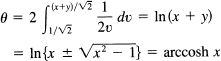
where since y > 0 for positive angles the plus sign is used. This is the arccosh x as we asserted at the end of Section 21.6. From this it follows that
x = cosh θ
which shows that the angle plays the same role for both types of functions.
Thus the hyperbolic functions can be related to the hyperbola as the trigonometric (circular) functions are related to the circle. The analogy is often useful. However, it should be noted that when you represent some function in terms of the sinh x and cosh x for large positive x you are in trouble, since the two functions are both approximately
![]()
While, mathematically, the two functions cosh x and sinh x are linearly independent, in the presence of roundoff errors they are practically dependent (for |x| large).
21.8 SUMMARY
In this chapter we have greatly extended the use of infinite series, especially power series. Since the power series is unique in any range, it follows that the powers of x are linearly independent for all powers, and we may equate the corresponding coefficients in two expressions that represent the same function in the same range. This is the basis for the generating function approach to many problems, especially combinatorial problems, where it is the main tool.
The binomial theorem was extended, by the usual approach, from integers to fractions, and then to all real exponents. Some tests of this new formula were given to both convince you that the formal expansions were consistent and to give you some practice in handling fractional exponents. Then a few of the numerous applications were indicated.
Next, we took on the tentative extension from the real numbers to the complex in the matter of power series. We simply asserted that the same formal power series we obtained for reals applied also for complex numbers. In particular, we used pure imaginary exponents to get the important Euler identities and found their relationship to the trigonometric functions. Thus we connected apparently different parts of mathematics together and found an inner unity. This phenomenon was discussed in Chapter
1 when we observed that the same kinds of things kept coming up in very different situations—the universality of mathematics. It follows that the inverse functions must similarly be related.
We then examined a close analogy to the trigonometric functions, called the hyperbolic functions. They again showed an inner structure that is not evident on the surface. This time we had to alter our original definition of angle to make the close analogy, something that should not surprise you. When you begin mathematics, there are often several ways of starting, several ways of defining things. As you progress and search for the inner unity, you sometimes have to go back and pick a different approach to make an analogy work. It is this inner unity, behind the surface diversity, that mathematicians find so beautiful about their subject. And this unity applies not only to pure mathematics, but often occurs in its various applications—the same mathematics is used in widely different fields. In a sense the mathematician is the last universalist; a sound knowledge of mathematics enables you to work in many different fields, and the contributions in your field are apt to reveal the unity behind the apparent diversity in many different fields of application.