This chapter deals with the last version of the memory allocation problem addressed in this book. The objective is to allocate data structures from a given application, to a given set of memory banks. In this variant, the execution time is split into time intervals. The memory allocation must consider the requirement and constraints at each time interval. Hence, the memory allocation is not static, it can be adjusted beause the application needs for data structures may change at each time interval.
After proposing an ILP model, we discuss two iterative metaheuristics for addressing this problem. These metaheuristics aim at determining which data structure should be stored in a cache memory at each time interval in order to minimize costs of reallocation and conflict. These approaches take advantage of metaheuristics designed for the previous memory allocation problem (see Chapters 3 and 4).
The dynamic memory allocation problem, called MemExplorer-Dynamic, is presented in this chapter. This problem has a special emphasis on time performance. The general objective is to allocate data structures for a specific application to a given set of memory banks.
This problem is related to the data binding problems (section 1.3.3). For instance, in the work presented in [MAR 03], a periodical set of data structures must be allocated to memory banks; thus, the objective is to minimize the transfer cost produced by moving data structures between memory banks. Despite these similarities, there is no equivalent problem to the dynamic memory allocation problem.
The main difference between MemExplorer and this dynamic version of the memory allocation problem is that the execution time is split into T time intervals whose durations may be different. Those durations are assumed to be given along with the application. During each time interval, the application requires accessing a given subset of its data structures for reading and/or writing.
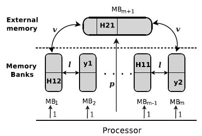
Figure 5.1 shows the memory architecture for MemExplorer-Dynamic, which is similar to that of a TI-C6201 device. It is composed of memory banks and an external memory. These memory banks have a limited capacity, and the capacity of external memory is large enough to allocate all data structures. The size of the data structures and the number of their accesses to them are both taken into account. Capacities of memory banks and the size of data structures are expressed in kilobytes (kB).
The processor accesses the data structure to perform the instructions of the application. As in MemExplorer, the access time of a data structure is its number of accesses multiplied by the transfer rate from the processor to memory banks or external memory. As before, the transfer rate from the processor to a memory bank is 1 ms, and the transfer time from processor to the external memory is p ms.
Figure 5.1. Memory architecture for MemExplorer
Initially (i.e. during time interval I0), all data structures are in the external memory and memory banks are empty. The time required for moving a data structure from the external memory to a memory bank (and vice versa) is equal to the size of the data structure multiplied by the transfer rate v ms per kilobyte (ms/kB). The time required for moving a data structure from a memory bank to another is the size of data structure multiplied by the transfer time between memory banks, l ms/kB.
The memory management system is equipped with a direct memory access (DMA) controller that allows for a direct access to data structures. The time performances of that controller are captured with the numerical values of v and l. Therefore, the transfer times v and l are assumed to be less than the transfer time p.
The TI-C6201 device can access all its memory bank simultaneously, which allows for parallel data loading. As in the previous chapters, two conflicting data structures, namely a and b, can be loaded in parallel, provided that a and b are allocated to two different memory banks. If these data structures share the same memory bank, the processor has to access them sequentially, which requires twice the amount time if a and b have the same size.
Each conflict has a cost equal to the number of times that it appears in the application during the current time interval. This cost might be a non-integer if the application source code has been analyzed by a code-profiling software [IVE 99, LEE 02], based on the stochastic analysis of the branching probability of conditional instructions. This happens when an operation is executed within a while loop or after a conditional instruction such as if or else if (see the example of the non-integer cost presented in Chapter 3).
As before, a conflict between two data structures is said to be closed if both data structures are allocated to two different memory banks. In any other case, the conflict is said to be open.
Moreover, both particular cases, auto-conflicts and isolated data structures, are considered in this version of memory allocation problem.
The number of memory banks with their capacities, the external memory and its transfer rate, p, v and l, describe the architecture of the chip. The number of time intervals, the number of data structures, their size and access time describe the application, whereas the conflicts and their costs carry information on both the architecture and the application.
Contrarily to MemExplorer, where a static data structure allocation is searched for, the problem addressed in this chapter is to find a dynamic memory allocation, that is the memory allocation of a data structure may vary over time. Roughly speaking, we want the right data structure to be present in the memory architecture at the right time, while minimizing the efforts for updating memory mapping at each time interval.
MemExplorer-Dynamic is stated as follows: allocate a memory bank or the external memory to any data structure of the application for each time interval, so as to minimize the time spent in accessing and moving data structures while satisfying the memory banks’ capacity.
The rest of the chapter is organized as follows. Section 5.2 gives an integer linear program formulation. Two iterative metaheuristics are then proposed for addressing larger problem instances in section 5.4. Computational results are then shown and discussed in section 5.5, and section 5.7 concludes this chapter.
Let n be the number of data structures in the application. The size of a data structure is denoted by si, for all i in {1,…,n}. nt is the number of data structures that the application has to access during the time interval It, for all t in {1…, T}. At ⊂ {1,…,n} denotes the set of data structures required in the time interval It for all t ∈ {1,…,T}. Thus, ei,t denotes the number of times that i ∈ At is accessed in the interval It. The number of conflicts in It is denoted by ot, and dk,t is the cost of conflict (k, t) = (k1, k2) during the time interval It for all k in {1,…, ot}, k1 and k2 in At, and t in {1,…,T}.
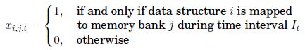
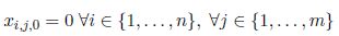
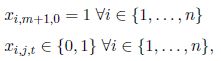
The allocation of data structures to memory banks (and to the external memory) for each time interval is modeled as follows. For all (i, j, t) in {1,…, n} × {1,…, m + 1} × {1,...., T},
The statuses of conflicts are represented as follows. For all k in {1,…, ot} and t ∈{1,…,T},
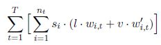
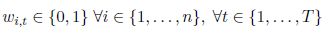
The allocation change for a data structure is represented with the two following sets of variables. For all i in {1,…,n} and t ∈ {1,…,T}, wi,t is set to 1 if and only if the data structure i has been moved from a memory bank j ≠ m + 1 at It–1 to a different memory bank j′ ≠ m + 1 during time interval It. For all i in {1,…,n} and t ∈ {1,…, T}, w′i,t is set to 1 if and only if the data structure i has been moved from a memory bank j ≠ m + 1 at It–1 to the external memory, or if it has been moved from the external memory at It–1 to a memory bank during time interval It.
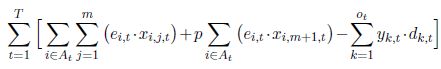
The cost of executing operations in the application can be written as follows:
The first term in [5.3] is the access cost of all the data structures that are in a memory bank, the second term is the access cost of all the data structures allocated to the external memory and the last term accounts for the closed conflict cost.
The total cost of moving data structures between the intervals can be written as:
The cost of a solution is the sum of these two costs. Because  is a constant term for all t in {1,…, T}, the cost function to minimize is equivalent to:
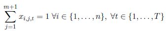
The ILP formulation of MemExplorer-Dynamic is then
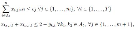
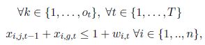
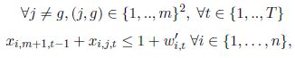
Equation [5.7] enforces that any data structure is either allocated to a memory bank or to the external memory. Equation [5.8] states that the total size of the data structures allocated to any memory bank must not exceed its capacity. For all conflicts (k, t) = (k1, k2), [5.9] ensures that data structure yk,t is set appropriately. Equations [5.10]–[5.12] enforce the same constraints for data structures wi,t and w′i,t. The fact that initially all the data structures are in the external memory is enforced by [5.13] and [5.14]. Finally, binary requirements are enforced by [5.15]–[5.18].
This ILP formulation has been integrated in SoftExplorer. It can be solved for modest size instances using an ILP solver such as Xpress-MP [FIC 09]. Indeed, as MemExplorer is NP-hard, and then is MemExplorer-Dynamic.
For the sake of illustration, MemExplorer-Dynamic is solved on an instance originating in the least mean square (LMS) dual-channel filter [BES 04], which is a well-known signal processing algorithm. This algorithm is written in C and is to be implemented on a TI-C6201 target. On that target, p = 16 ms, and l = v = 1 ms/kB.
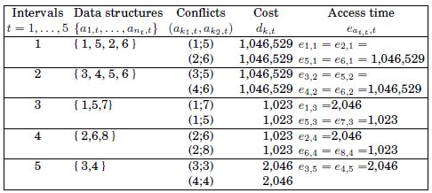
The compilation and code profiling of the C file yields an instance with eight data structures having the same size of 15,700 kB; there are two memory banks whose capacity is 31,400 kB. For each time interval, Table 5.1 displays the data structures required by the application, the access time, the conflicts and their cost.
Table 5.1. Data about LMS dual-channel filter
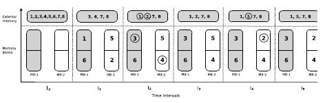
An optimal solution found by Xpress-MP [FIC 09] is shown in Figure 5.2. All data structures are in the external memory in initial interval I0. In the first interval no conflict is open, only the moving cost is produced. A memory bank can only store two data structures. In the second time interval, data structures 1, 2, 3 and 4 are swapped for avoiding access to data structures 3 and 4 from the external memory. Thus, no open conflict is produced, but a moving cost is generated. The memory allocation remains the same for the third interval, so a non-moving cost is produced but the conflict between data structures 1 and 7 is open. The optimal solution does not swap any data structures because they are used in the future intervals; in this way, the future moving cost is saved. In the fourth interval, data structures 5 and 2 are swapped, so no conflict is open, a moving cost is produced and the access time of data structure 8 is longer (p × e8,4). For the last time interval, the memory allocation remains the same, and the cost of the auto-conflicts is generated.
Figure 5.2. An optimal Solution for the example of MemExplorer-Dynamic
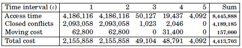
The cost of this solution is 4,413,703 ms. Table 5.2 shows how this cost is dispatched. For each time interval, this table displays: the time spent by accessing data structures, the cost produced by moving data structures and the saved cost produced by closed conflicts.
Table 5.2. Cost of the optimal solution for the example of MemExplorer-Dynamic
For larger instances (i.e. with more data structures, more conflicts, more memory banks and more time intervals), the proposed ILP approach can no longer be used. In the following section, two iterative metaheuristics are proposed for addressing MemExplorer-Dynamic.
This approach takes into account the application requirements for the current and future time intervals. The long-term approach relies on addressing the general memory allocation (see Chapter 4). MemExplorer searches for a static memory allocation of data structures that could remain valid from the current time interval to the end of the last time interval. MemExplorer ignores the fact that the allocation of data structures can change at each time interval.
The long-term approach builds a solution iteratively, that is from time interval I1 to time interval IT. At each time interval, it builds a preliminary solution called the parent solution. The solution for the considered time interval is built as follows: the solution is initialized to the parent solution. Then, the data structures that are not required until the current time interval are allocated to the external memory.
At each time interval, the parent solution is selected from two candidate solutions. The candidate solutions are the parent solutions for the previous interval, and the solution to MemExplorer for the current interval. MemExplorer is addressed using a variable neighborhood search-based approach hybridized with a tabu search-inspired method (see Chapter 4).
The total cost of both candidate solutions is then computed. This cost is the sum of two subcosts. The first subcost is the cost that we would pay if the candidate solution were applied from the current time interval to the last time interval. The second subcost is the cost to be paid for changing the memory mapping from the solution of the previous time interval (which is known) to the candidate solution. Then, the candidate solution associated with the minimum total cost is selected as the parent solution.
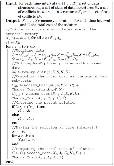
The long-term approach is presented in Algorithm 13. A memory allocation is denoted by X, X(a) = j, means that data structure a is allocated to memory bank j. The solution Xt is associated with time interval It for all t in {1,…, T}. The solution X0 consists in allocating all the data structures of the application to the external memory.
The parent solution is denoted by Pt for the time interval It. The algorithm builds the solution Xt by initializing Xt to Pt, and the data structures that are not required until time interval It is moved to the external memory.
In the algorithm, Mt is the memory allocation found by solving the instance of MemExplorer built from the data for the time interval It. Then, a new instance of MemExplorer is solved at each iteration.
Algorithm 13 uses two functions to compute the total cost of a solution X. The first subcost is computed by the function Access_Cost(). This function returns the cost produced by a memory allocation X for a specified instances (data) of MemExplorer. The second subcost is computed by the function Change_Cost(X1, X2). It computes the cost of changing solution X1 into solution X2.
At each time interval It, the parent solution Pt is chosen between two candidates Pt–1 and Mt.This parent solution produces the minimum total cost (comparing both the total cost CPt–1 and CMt).
At each iteration, Algorithm 13 updates the data and uses the same process to generate the time interval solution Xt for all t in {1,…,t}.
Algorithm 13. Long-term approach
This approach relies on addressing a memory allocation subproblem called MemExplorer-Prime. Given an initial memory allocation, this subproblem is to search for a memory allocation of the data structures that should be valid from the current time interval. This subproblem takes into account the cost for changing the solution of the previous time interval.
Algorithm 14. Short-term approach
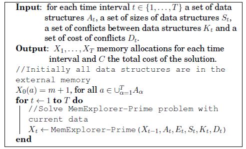
MemExplorer-Prime is addressed for all time intervals. The data of this subproblem are the same as for MemExplorer. MemExplorer-Prime is stated as follows: for a given initial memory allocation for data structures, the number of capacitated memory banks and an external memory, we search for a memory allocation such that the time spent accessing data and the cost of changing allocation of these data are minimized. In this chapter, MemExplorer-Prime is addressed using a tabu search method similar to the method used by the long-term approach.
The short-term approach iteratively builds a solution for each time interval. Each solution is computed by taking into account the conflicts and data structures involved in the current time interval, and also by considering the allocation in the previous time interval. The short-term approach solves MemExplorer-Prime considering the allocation of the data structures of the previous interval as an initial allocation.
Algorithm 14 presents this approach. A solution X is defined as above, and it uses a function MemExplorer-Prime() for solving an instance of the problem MemExplorer-Prime where the initial solution is X0.
At each iteration, the algorithm updates the data and the solution produced by MemExplorer-Prime() is taken as the time interval solution.
This section presents the results obtained by the iterative approaches, which have been implemented in C++ and compiled with gcc4.11 in Linux OS 10.04. They have been tested over two sets of instances on an Intel® Pentium IV processor system at 3 GHz with 1 GB RAM. The results produced by the iterative approaches are compared with the results of the ILP model and the local search method.
In practice, softwares such as SoftExplorer [LAB 06] can be used for collecting the data, but the code profiling is out of the scope of this work. We have used 44 instances to test our approaches. The instances of the set LBS are real-life instances that come from electronic design problems addressed in the LAB-STICC laboratory. The instances of DMC come from DIMACS [POR 09a], a well-known collection of graph coloring instances. The instances in DMC have been enriched by generating some edge costs at random to represent conflicts, access costs and sizes for data structures, the number of memory banks with random capacities and by dividing the conflicts and data structures into different time intervals.
For assessing the practical use of our approaches for forthcoming needs, we have tested our approaches on larger artificial instances, because the real-life instances available today are relatively small. In the future, the real-life instances will be larger and larger because designers tend to integrate more and more complex functionalities in embedded systems.
For the experimental test, we have set the following values for transfer times: p = 16 (ms), and l = v = 1 (ms/kB) for all instances.
In Table 5.3, we compare the performances of the different approaches with the local search produced by LocalSolver 1.0 [INN 10] and with the ILP formulation solved by Xpress-MP, that is used as a heuristic when the time limit of one hour is reached: the best solution found so far is then returned by the solver.
We presented the instances sorted by non-decreasing sizes (i.e. by the number of conflicts and data structures). The first two columns of Table 5.3 show the main features of the instances: name, number of data structures, conflicts, memory banks and time intervals. The next two columns display the cost and the CPU time of the short-term approach in seconds (s). For the long-term approach, we show the best costs and its time reached in 12 runs, the standard deviation and the ratio between the standard deviation and average cost. For the local search, the cost and CPU time are also displayed. The following two columns report the cost and CPU time of the ILP approach. The column “gap” reports the gap between the long-term approach and the ILP. It is the difference of costs of the long-term approach and the ILP divided by the cost of ILP. The last column indicates whether the solution returned by Xpress-MP is optimal.
The optimal solution is known only for the smallest instances. Memory issues prevented Xpress-MP and LocalSolver to address the nine largest instances. It is the same case for the LocalSolver, its memory prevents to address six of the largest instance.
Bold figures in the table are the best known solutions reported by each method. When the optimal solution is known, only three instances resist the long-term approach with a gap of at most 3%. From the 17 instances solved by Xpress-MP but without guarantee of the optimal solution, the ILP method finds six best solutions whereas the long-term approach improves 11 solutions, even sometimes up to 48%.
The last three rows of the table summarize the results. The short-term approach finds four optimal solutions and the long-term approach finds 14 of the 18 known optimal solutions. The local search reaches six optimal solutions. The long-term approach is giving the largest number of best solutions with an average improvement of 6% over the ILP method.
The practical difficulty of an instance is related to its size (n, o), but it is not the only factor. The ratio between the total capacity of the memory bank and the sum of the sizes of data structures also plays a role. For example, instances mug88_1dy and mug88_25dy have the same size but the performance of Xpress-MP for the ILP formulation is very different.
Table 5.3. Cost and CPU time for MemExplorer-Dynamic


In most cases, the proposed metaheuristic approaches are significantly faster than Xpress-MP and LocalSolver, with the short-term approach being the fastest approach. The short-term approach is useful when the cost of reallocating data structures is small compared to conflicts costs. In such a case, it makes sense to focus on minimizing the cost of the current time interval without taking future needs into account, because the most important term in the total cost is due to open conflicts. The long-term approach is useful in the opposite situation (i.e. moving data structures is costly compared to conflict costs). In that case, anticipating future needs makes sense as the solution is expected to undergo very few modification over time. Table 5.3 shows that the architecture used and the considered instances are such that the long-term approach returns a solution of higher quality than the short-term approach (except for r125.1cdy), and then emerges as the best method for today’s electronic applications, as well as for future needs.
As in the previous chapter, we used the Friedman test [FRI 37] to identify differences in the performance of iterative approaches, local search and ILP solution. The post hoc paired test is also performed to identify the best approach.
For this test, we use the results presented in Table 5.3, because the results over instances are mutually independent. Thus, costs as well as CPU times can be ranked as in Chapter 4, and the Friedman test statistic is denoted by Q and it is defined as in equation [4.10].
The test statistic Q is 18.85 for the objective function, and 111.18 for the CPU time. Moreover, the value for the F(3,102)-distribution with a significance level α = 0.01 is 3.98. Then, we reject the null hypothesis for cost and running time at the level of significance α = 0.01.
Hence, we conclude that there exists at least one metaheuristic whose performance is different from at least one of the other metaheuristics.
We use the same post hoc test of section 4.6 for comparing the performance between two metaheuristics. Table 5.4 summarizes the paired comparisons for the cost and running time using an α = 0.01; thus, t(0.095,102)-distribution is 2.63, and the left-hand side of equation [4.11] for the running time is 13.21 and the cost is 21.26. Data given in bold highlights the best obtained results.
Table 5.4. Paired comparisons for MemExplorer-Dynamic
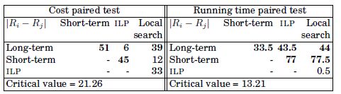
The post hoc test shows that the ILP and the long-term approach have the same performance in terms of solution cost, but the long-term approach is better than the ILP in terms of running time. The long-term approach outperforms the local search and short-term approach. On the other hand, the short-term approach is the best approach in terms of running time and its performance in terms of cost is equal to the one of local search. Finally, ILP and local search have the same performance in terms of running time.
This chapter presents an exact approach and two iterative metaheuristics, based on the general memory allocation problem. Numerical results show that the long-term approach gives good results in a reasonable amount of time, which makes this approach appropriate for today’s and tomorrow’s needs. However, the long-term approach is outperformed by the short-term approach in some instances, which suggests that taking the future requirements and aggregating the data structures and conflicts of the forthcoming time interval might not always be relevant. In fact, the main drawback of this approach is that it ignores the potential for updating the solution at each iteration.
The work discussed in this chapter has been presented at the European Conference on Evolutionary Computation in Combinatorial Optimization (EVOCOP) [SOT 11c].