Chapter 20. Sampling Plant Populations in a Community
Equipment and Materials
You’ll need the following items to complete this field session. (The standard kit for this book, available from www.thehomescientist.com, includes the items listed in the first group.)
Materials from Kit
Centrifuge tubes (specimen containers)
Magnifier
Ruler
Materials You Provide
Gloves
Assistant
Camera (optional, with macro feature)
Hammer or mallet
Marking pen (for labeling)
Field guides to plants and trees (for your region)
Plastic bags (specimen containers)
Pocket knife
Scissors
Stakes (see text)
String or cord (250 feet or 75 meters)
Tape measure (50-foot or 15-meter)
Background
In this field session we’ll define a survey area and do sample counts of the plant populations within that area. From those sample counts, we’ll estimate plant populations for the area as a whole.
Such population surveys are an important tool for ecologists, who use them to track the rise and fall in populations of various species in the environment. Like a canary in a coal mine, the rise or decline in population of a species that is particularly sensitive to a particular environmental factor may provide an early warning of significant environmental changes that otherwise may not have been detected until months, years, or even decades later.
Other than collecting household items, no advance preparation is required for any of the procedures in this field session. You can save time in the field by preparing four 10-meter (32’ 13/16”) lengths and 16 one-meter (39-3/8”) lengths of cord ahead of time. Tie loops large enough to fit over the stakes in both ends of each cord, ensuring that the cords are the proper length when stretched from the end of one loop to the end of the other.
Note
Although this field session focuses on surveying plant populations in a community, you can also take advantage of this field trip to gather other specimens, such as fungi, insects, and even animals. (Always know and abide by your local laws and regulations pertaining to contact with wildlife.)
Wildlife is not defenseless, as anyone who has encountered hornets or poison ivy can attest. Always wear gloves, goggles, and protective clothing when you gather specimens, and always know what specimens you are gathering. Capturing a garter snake for your terrarium is one thing; mistaking a water moccasin for a garter snake is quite another.
Procedure V-1-1: Choosing and Preparing the Survey Area
In this procedure, we’ll select and prepare a defined area for observing plant populations within a community. Choose an area with considerable diversity in plants. For example, a well-maintained lawn is a poor choice because the flora are predominantly one species. In suburban areas, a park or natural area often provides many suitable locations.
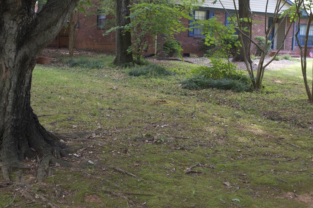
Try to choose an area that has a mixture of trees, shrubs, grasses, and ground cover (lichens, mosses, etc.) An area that has parts that are usually shaded and others that are often sunlit usually provides considerably more diversity than an area that is exclusively shaded or sunlit. A sampling area that is on the boundary between a wooded area and a grassy area often provides more diversity than is common in residential areas. Figure 20-1 shows part of the survey area we chose.
Having chosen the survey area, make sure you have permission to use it. Over the course of a couple hours or more, you will be driving stakes and possibly shooting images and taking plant specimens. Many property owners will freely give permission, particularly if you explain the purpose of your activities and promise to clean up afterward, but some will not.
Warning
You will be observing and handling wild plants. Wear gloves to prevent toxic or irritating plants from contacting your skin. Do not disturb animal or insect nests. Do not gather specimens that you cannot identify at least generally. Wash your hands thoroughly after handling plant specimens.
Once you have permission to use the area, proceed as follows:
Choose a section of the area that you expect to exhibit considerable species diversity and is 10 meters or more square.
Drive stake #1 at one corner of the area you have selected. Measure 10 meters (32’ 13/16”) along one side of the square you’ve chosen and drive stake #2 at that point to form the first side of the square. Stretch one of your 10-meter cords between stakes #1 and #2.
Note
You can use plant stakes from the garden store, or anything similar that is large enough and strong enough to secure the cord on the corners of the square. For example, tent pegs or large nails are suitable. If nothing else is available, you can use short sections of small fallen branches.
We’ll use geometry to ensure that our square is really square. The diagonal of a square is 1.414 times the length of a side, so all we need to do is make sure the 14.14 meter diagonal and the next 10 meter side meet at the same point.
Loop a second 10-meter cord over stake #2, and stretch it out to about where stake #3 should be placed. Have your assistant hold the free end of the tape measure on stake #1, and pull the tape out to 14.14 meters (14 m, 14 cm or 46’ 3/8”). The point where the end of the 10-meter cord and the 14.14 meter mark on the tape measure meet is the next corner of the square. Drive stake #3 at that point, and place the loop on the free end of cord #2 over that stake. (It is not necessary to be exact, but keep as close as you can to a true square that’s 10 meters on a side.)
Repeat step 3, placing one end of another 10-meter cord on stake #3 and stretching the cord out to about where the final corner of the square should be. Have your assistant hold the free end of the tape measure on stake #2, and pull the tape out to 14.14 meters. The point where the end of the 10-meter cord and the 14.14 meter mark on the tape measure meet is the final corner of the square. Drive stake #4 at that point and place the loop on the free end of cord #3 over the stake. Finally, use cord #4 to connect stakes #4 and #1, completing the square.
Procedure V-1-2: Surveying the Plant Community
After defining the survey area, the next procedure is to locate and identify as many plant species as possible within this defined area. If you have chosen your area well, you should be able to locate at least half a dozen plant species within the survey area, and possibly many more. (We identified more than two dozen species in our own survey area.)
Look for plants in the following categories:
Woody plants – trees, shrubs, and vines
Herbaceous plants – grasses, weeds, small flowering plants
Ground cover – mosses, worts, and lichens (lichens are technically not plants)
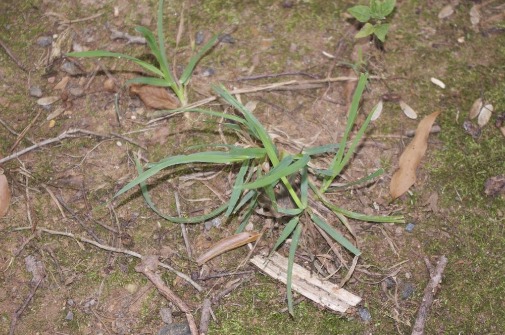
Plants representing all three of these categories were present in our own survey area, and will likely be present in your survey area as well. Representatives of two of these categories are readily visible in Figure 20-1, the trees (woody plants) and the green ground covering (a moss). Figure 20-2 shows a representative herbaceous plant.
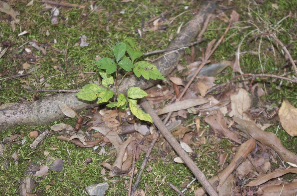
As you perform your survey, keep in mind that specimens of the same species at different life stages may have different appearances. For example, although they appear very different, the small plant shown in Figure 20-3 is actually a juvenile example of Acer cappadocium ‘Aureum’, the golden maple tree shown on the left in Figure 20-1.
How do we know? Well, not being botanists, we couldn’t swear to it. (Even botanists can’t necessarily identify specimens absolutely by visual means alone.) But there is some strong evidence to suggest that this juvenile plant is in fact Acer cappadocium ‘Aureum’. First, it is growing within the roots of an adult golden maple. We’re reasonably certain of the species (Acer cappadocium) and cultivar (‘Aureum’) of the adult tree because its leaves are five- and seven-lobed (versus the three- or five-lobed leaves of the Acer rubrum (red maple) trees that also grow in the immediate vicinity, and because we have watched that tree’s leaves change to a brilliant golden color every autumn for the last 20 years (rather than the bright reds and oranges of Acer rubrum). The fact that the large upper right leaf of the juvenile plant exhibits seven nodes makes the identification nearly conclusive.
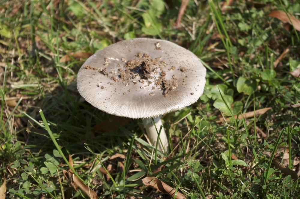
As you do your survey, also log any plant-like lifeforms you observe. For example, we logged the magnificent example of the fungi Amanita sp. shown in Figure 20-4. The cap of this specimen was about 10 cm in diameter. Such fungi can disappear literally overnight, so we also took a sample for later microscopic analysis.
Warning
Treat all mushrooms as potentially lethal. Many species of Amanita are among the most poisonous flora known. Handle them only with gloves, do not inhale the spores, and never under any circumstance eat mushrooms that you have picked yourself. Even expert mycologists have died from consuming misidentified mushrooms.
As you encounter each species, use the guidebooks to identify it. Record the identity of each species, along with your notes about its size and other pertinent characteristics in your lab notebook. If you have a camera, record images of each of the species for your records. (You can provide scale within the image simply by including a ruler in the image.) If possible, shoot multiple images of each specimen, including close-up images that show details such as leaf structure. In particular, photographically document any species that you cannot identify with specificity using the guidebooks.
If you have time (and permission), where practical gather specimens of each species, or at least of a representative sample. (No, we don’t expect you to carry home a tree...) If it is not practical to obtain a whole specimen, obtain leaves, flowers, seeds, or other parts of the plant. For small lifeforms (such as mosses), cut or dig up a small representative specimen. Store these specimens in tubes or plastic bags, and observe them in more detail when you get home.
Note
Use tubes or plastic bags only for temporary storage, when you want to prevent a specimen from drying out. If you want to preserve specimens (such as mosses, lichens, flowers, and so on) long-term, do not store them in sealed containers, which retain water and will allow the specimen to decay. Instead, store such specimens in paper bags, cardboard boxes, or similar containers that will allow water vapor to escape.
Procedure V-1-3: Performing a Population Count
Biologists make population counts to record and track the numbers of specific species present in an area, and to determine the changes in those populations over time. The appropriate size for the survey area depends on the size and numbers of the species being surveyed. Our survey area is a square 10 meters on a side or 100 m2, which is appropriate for medium-size species that are present in moderate numbers. If were were surveying a larger and less common species—oak trees, for example—we might choose a survey area 1,000 meters on a side, or 1 km2. If we were surveying a small species that was present in large numbers, we might choose a survey area one meter on a side, or even 10 cm on a side.
If—and this is critically important—the selected survey area is representative of the area as a whole, we can determine the population of the species in the survey area and extend that by multiplication to determine the population numbers for the larger area of which the survey area is a part. For example, we might determine the population of Aconitum sp. (monkshood) plants in a survey area 100 meters on a side (0.01 km2) is 22 individuals. From this data, we could estimate the population of monkshood plants in a larger surrounding area of 1,000 meters on a side (1 km2) as 2,200 individuals.
Warning
If you do have monkshood plants in your survey area, use extreme caution. Monkshood contains significant amounts of aconitine, one of the deadliest alkaloid poisons known. The lethal dose of aconitine for an adult human is usually stated as between 3 and 6 milligrams (about 1% of the mass of an aspirin tablet), so ingesting even a few grams of the monkshood plant may be lethal. Nor is monkshood the only deadly plant commonly found in residential yards and flower gardens. Again, use extreme caution in handling plant specimens.
But such estimates are inherently imprecise, because it’s impossible to state with certainty that the survey area is really representative of the surrounding area as a whole. We might, for example, have chosen entirely by coincidence the one 0.01 km2 area in that larger area that contained any monkshood plants at all.
To reduce the uncertainty inherent in such estimates, biologists sample multiple survey areas (called quadrats) within the larger area. For example, rather than counting the population in only one 0.01 km2 survey area within the larger 1 km2 area—which is to say only 1% of the larger area—a biologist might randomly choose five 0.01 km2 survey areas within the larger area. And the “randomly” part is important in reducing uncertainty.
In this procedure, we’ll establish four 1m2 quadrats within the survey area, do population counts of each species for each quadrat, and extend our results to estimate the population of that species in the entire survey area. Although it won’t be random in a strict mathematical sense, we’ll establish our four 1 m2 quadrats simply by measuring specific lengths on the 10-meter lines that define the survey area. (For a distribution closer to actual random, you can stand several meters outside your large survey area with your back to it, and toss an object over your shoulder. Wherever that object lands within the survey area is the center of your first 1 m2 quadrat; repeat the process to define the remaining three quadrats.
Use the measuring tape and marking pen to make four marks on each of two 10-meter cords that are opposite sides of the square. Place marks on each cord at two meters and three meters from each end. That is, each cord should be marked along its length at the following points: 2, 3, 7, and 8 meters.
Extend the tape measure between two of the marks directly opposite each other, and drive in stakes at the 2, 3, 7, and 8 meter marks of the measuring tape.
Repeat step 2 for each of the other three marks on the two 10-meter cords. When you have finished, you should have 16 stakes driven inside the survey area, forming four squares, each one meter on a side. Wrap cord around each of those four sets of stakes to define the four 1 m2 quadrats.
Referring to your notes, count the number of individuals present in the first quadrat for each of the species you found within the larger survey area. For discrete plants, count the actual number within the quadrat. (If a plant lies exactly on the quadrat border, count it as 0.5.) For grasses, mosses, and other ground cover plants, where it is difficult to discriminate individuals, estimate as closely as possible the percentage of the quadrat surface area covered by that plant.
Repeat step 4 for each of the remaining quadrats.
Using the data you obtain from the quadrat counts, estimate the population of each species within the larger survey area.
Review Questions
Q1: Why did we do counts in four quadrats rather than just one? Why did we not use 3, 5, or (say) 17 quadrats?
Q2: How did you calculate the estimated population of each species within the survey area?
Q3: Were all three plant categories (woody plants, herbaceous plants, ground cover) represented in your survey area? Which were the most and least common? Which was the dominant species?
Q4: Did the species counts differ significantly among the four quadrats? If so, what reasons can you propose for the differences?
Q5: If you returned to the survey area and repeated the population count in one month, what changes (if any) would you expect? Six months? One year?
Q6: If a significant change to the survey area occurred, what effect would you expect? (For example, imagine that the tree in our survey area was cut down.)


