The first thing to know about charts is this:
Any chart, no matter how well designed, will mislead us if we don’t pay attention to it.
What happens after we do pay attention to a chart, though? We need to be able to read it. Before we learn how charts lie, we must learn how they are supposed to work when they are appropriately built.
Charts—also called visualizations—are based on a grammar, a vocabulary of symbols, and plenty of conventions. Studying them will immunize us against many abuses.
Let’s begin with the basics.
The year 1786 saw the publication of a most unusual book with what seemed to be an ill-fitting title: The Commercial and Political Atlas, by polymath William Playfair. “An atlas?” readers at the time may have wondered while browsing through its pages. “This book doesn’t contain any map whatsoever!” But it did. One of Playfair’s graphics can be seen below.
You probably have identified this chart as a common line chart, also called a time-series line graph. The horizontal axis is years, the vertical axis measures a magnitude, and the two lines waving through the picture represent the variation of that magnitude. The darker line (on top) is exports from England to other countries, and the lighter line is imports into England. The shaded area in between the lines emphasizes the balance of trade, the difference between exports and imports.
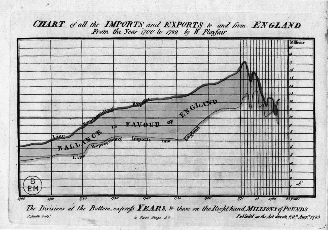
Explaining how to read a chart like this may seem unnecessary nowadays. My eight-year-old daughter, now in third grade, is used to seeing them. But that wasn’t the case at the end of the eighteenth century. Playfair’s Atlas was the first book to systematically depict numbers through charts, so he devoted plenty of space to verbalizing what readers were seeing.
Playfair wrote his explanations because he knew that charts are rarely intuitive at a quick glance: like written language, they are based on symbols, the rules (syntax or grammar), which guide how to arrange those symbols so they can carry meaning, and the meaning itself (semantics). You can’t decode a chart if you don’t grasp its vocabulary or its syntax, or if you can’t make the right inferences based on what you’re looking at.
Playfair’s book contains the word “atlas” because it truly is an atlas. Its maps may not represent geographic locations, but they are based on principles borrowed from traditional mapmaking and geometry.
Think of how we locate any point on the surface of the world. We do it by figuring out its coordinates, longitude and latitude. For instance, the Statue of Liberty is located 40.7 degrees north of the equator, and 74 degrees west of the Greenwich meridian. To plot its position, I simply need a map on which I can overlay a grid of subdivisions over the horizontal axis (the longitude) and vertical axis (the latitude):
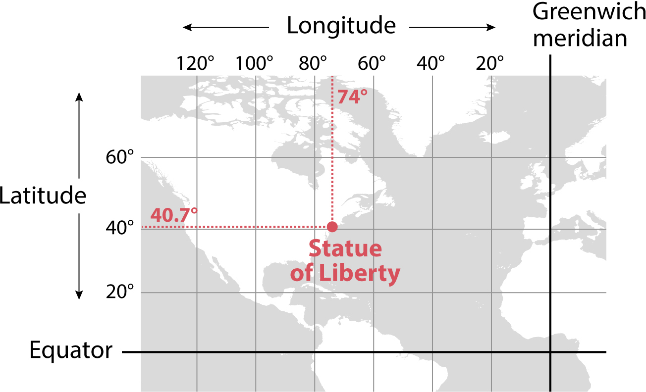
Playfair’s insight, which led him to create the first line graphs and bar graphs, was this: as longitude and latitude are quantities, they can be substituted by any other quantity. For instance, year is used instead of longitude (horizontal axis), and exports/imports instead of latitude (vertical axis).
Playfair employed a couple of simple elements that lie at the core of how most charts work: the scaffolding of a chart and its methods of visual encoding.

This is where I get a bit technical, but I promise that the little extra effort this chapter requires will pay off later. Moreover, what I’ll explain will prepare you for most of the charts you see anywhere and everywhere. Bear with me. Your patience will be rewarded.
To read a chart well, you must focus on the features that surround the content and support it—the chart’s scaffolding—and on the content itself—how the data is represented, or encoded.
The scaffolding consists of features such as titles, legends, scales, bylines (who made the graphic?), sources (where did the information come from?), and so forth. It’s critical to read them carefully to grasp what the chart is about, what is being measured, and how it’s being measured. Here are some examples of charts with their content displayed with and without scaffolding:

The scaffolding of the map includes a legend based on sequential shades of color, which indicate a higher murder rate (darker shades) or a smaller one (lighter shades). The scaffolding of the line graph is made of a title, a subtitle indicating the unit of measurement (“rate per 100,000 people”), labels on the horizontal and vertical scales to help you compare the years, and the source of the data.
Sometimes, short textual notes may supplement a chart, emphasizing or clarifying some important points. (Imagine that I had added the explainer “Louisiana has the highest murder rate in the United States, 11.8 per 100,000 people.”) We call this the “annotation layer,” a term coined by designers who work for the graphics desk of the New York Times. The annotation layer is also part of a chart’s content.
The core element of most charts is their visual encodings. Charts are always built with symbols—usually, but not always, geometric: rectangles, circles, and the like—that have some of their properties varied according to the numbers they represent. The property that we choose to change depending on our data is the encoding.
Think of a bar graph. In it, bar length or height varies in proportion to underlying numbers; the bigger the number, the longer—or taller—the bar will be:
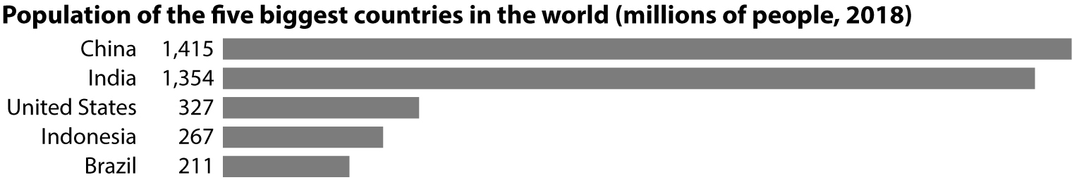
Compare India and the United States. The population of India is roughly four times the size of the U.S. population. Therefore, as our chosen method of encoding is length, India’s bar must be four times the length of that of the United States.
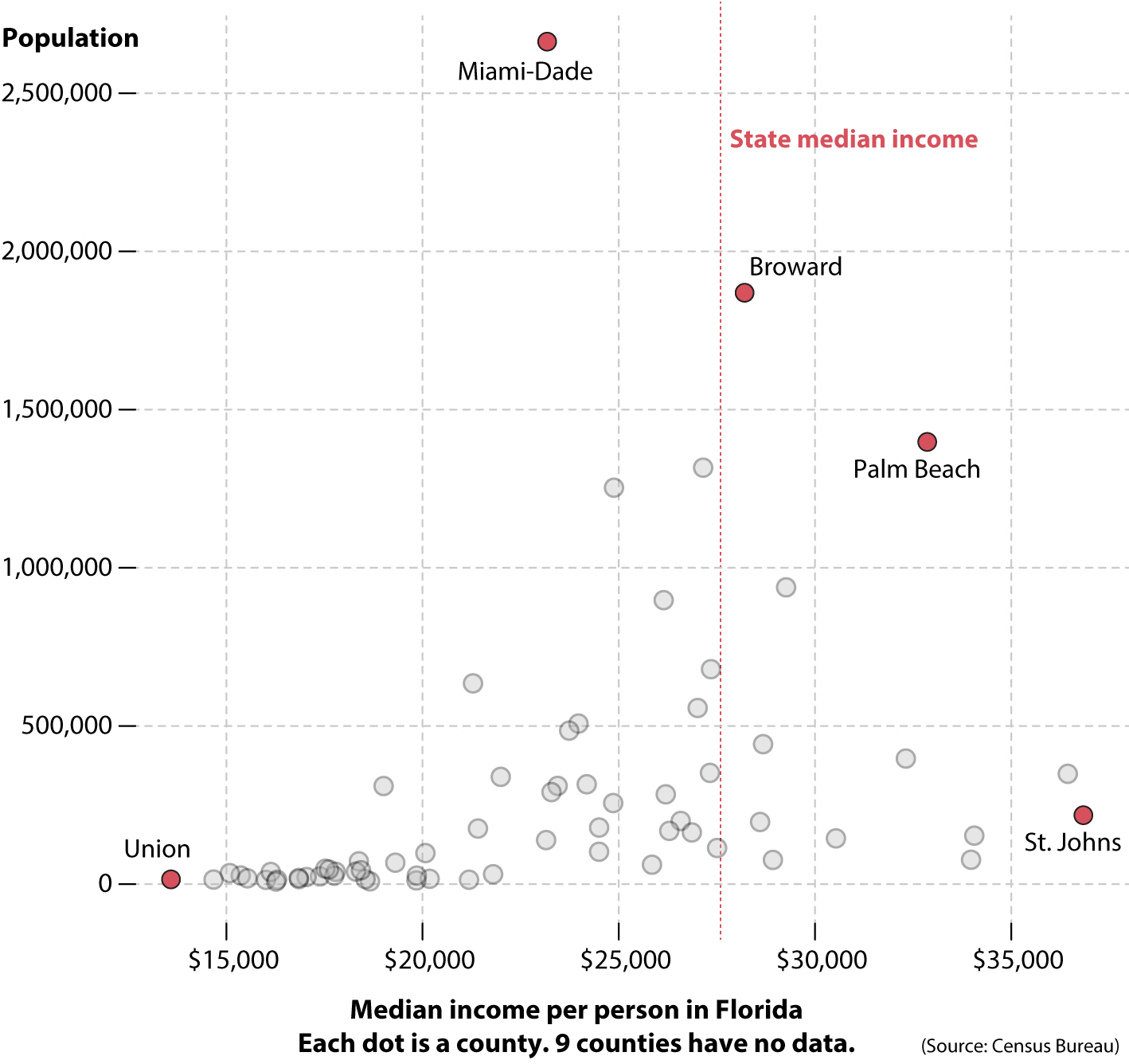
There are many other encodings that can be used in charts in addition to length or height. One very popular method is position. In the chart below, the position of each county in Florida—symbolized by a dot—on the horizontal (x) axis corresponds to the yearly income per person. The farther a dot is to the right, the richer the typical individual is in that county:
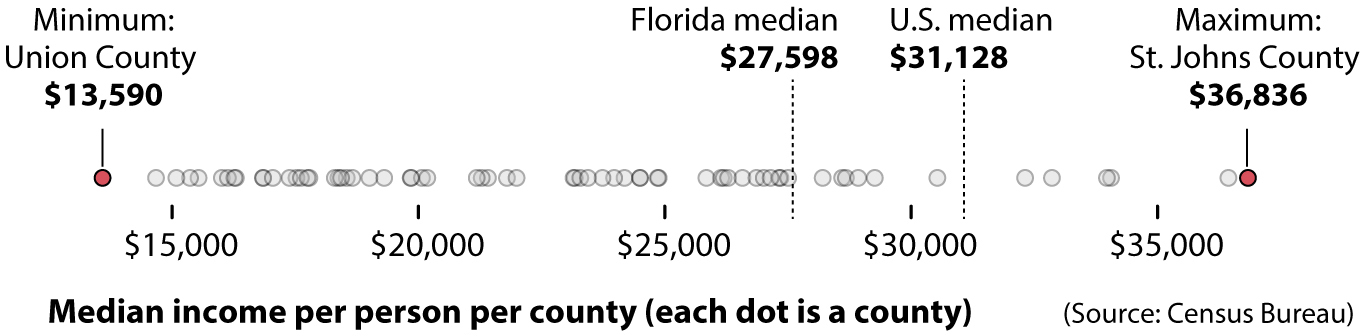
This chart compares the median income in each Florida county. The median is the score that splits the full range of values into two halves of equal size. Here’s an example: Union County has a median income of $13,590. Its population is roughly 15,000. Therefore, what the median tells us is that around 7,500 people living in Union County make more than $13,590 every year and the other 7,500 make less—but we don’t know how much more or less: some people may have an income of $0, and others may make millions.
Why are we using the median and not the more widely known arithmetic mean, also known as the average? We do this because the mean is very sensitive to extreme values and, as such, is much higher than typical incomes. Imagine this situation: You want to study the incomes of a county with 100 inhabitants. Ninety-nine of them have a yearly income very close to $13,590. But one of them makes $1 million a year.
The median of this distribution would still be $13,590: half the people are a bit poorer than that, and the other half—the half that includes our very wealthy friend—are richer. But the mean would be much higher: $23,454. This is the result of adding up the incomes of all inhabitants in the county and dividing the result by 100 people. As the old saying goes, whenever Bill Gates participates in a meeting, everyone in the room becomes a millionaire, if we take the arithmetic mean of the group’s wealth.
Let’s return to my dot chart. A large chunk of our brains is devoted to processing information that our eyes gather. That is why it’s often easier to spot interesting features of numbers when those numbers are represented through visual encodings. Take a look at the numerical table—a kind of chart, but not one that uses visual encodings—with all Florida counties and their corresponding median incomes.
County |
Income per person ($) |
Alachua County |
24,857 |
Baker County |
19,852 |
Bay County |
24,498 |
Bradford County |
17,749 |
Brevard County |
27,009 |
Broward County |
28,205 |
Calhoun County |
14,675 |
Charlotte County |
26,286 |
Citrus County |
23,148 |
Clay County |
26,577 |
Collier County |
36,439 |
Columbia County |
19,306 |
DeSoto County |
15,088 |
Dixie County |
16,851 |
Duval County |
26,143 |
Escambia County |
23,441 |
Flagler County |
24,497 |
Franklin County |
19,843 |
Gadsden County |
17,615 |
Gilchrist County |
20,180 |
Glades County |
16,011 |
Gulf County |
18,546 |
Florida median |
27,598 |
U.S. median |
31,128 |
Hamilton County |
16,295 |
Hardee County |
15,366 |
Hendry County |
16,133 |
Hernando County |
21,411 |
Highlands County |
20,072 |
Hillsborough County |
27,149 |
Holmes County |
16,845 |
Indian River County |
30,532 |
Jackson County |
17,525 |
Jefferson County |
21,184 |
Lafayette County |
18,660 |
Lake County |
24,183 |
Lee County |
27,348 |
Leon County |
26,196 |
Levy County |
18,304 |
Liberty County |
16,266 |
Madison County |
15,538 |
Manatee County |
27,322 |
Marion County |
21,992 |
Martin County |
34,057 |
Miami-Dade County |
23,174 |
Monroe County |
33,974 |
Nassau County |
28,926 |
Okaloosa County |
28,600 |
Okeechobee County |
17,787 |
Orange County |
24,877 |
Osceola County |
19,007 |
Palm Beach County |
32,858 |
Pasco County |
23,736 |
Pinellas County |
29,262 |
Polk County |
21,285 |
Putnam County |
18,377 |
St. Johns County |
36,836 |
St. Lucie County |
23,285 |
Santa Rosa County |
26,861 |
Sarasota County |
32,313 |
Seminole County |
28,675 |
Sumter County |
27,504 |
Suwannee County |
18,431 |
Taylor County |
17,045 |
Union County |
13,590 |
Volusia County |
23,973 |
Wakulla County |
21,797 |
Walton County |
25,845 |
Washington County |
17,385 |
Tables are great when we want to identify specific individual figures, like the median income of one or two counties, but not when what we need is a bird’s-eye view of all those counties together.
To see my point, notice how much easier it is to spot the following features of the data by looking at the dot chart rather than at the numerical table:
•The minimum and maximum values can be seen in comparison to the rest.
•Most counties in Florida have a lower median income than the rest of the United States.
•There are two counties, St. Johns and another one that I didn’t label, where the median income is clearly much higher than in the rest of Florida.
•There is one county, Union, that is much poorer than the other poor counties in Florida. Notice that there’s a gap between the position of Union County’s circle and the rest of the circles.
•There are many more counties with low median incomes than counties with high incomes.
•There are many more counties below the state’s median income ($27,598) than above it.
How is this last point possible? After all, I’ve just told you that the median is the value that splits the population in half. If that’s true, half the counties on my chart should be poorer than the state median, and the other half should be richer, shouldn’t they?
But that’s not how this works. That number of $27,598 is not the median of the medians of the 67 Florida counties. It’s the median income of the more than 20 million Floridians, regardless of the counties where they live. Therefore, it’s half the people in Florida (not half the counties) who make less than $27,598 a year, while the other half make more.
This apparent distortion on the chart might happen because of population size differences between counties that tend to be richer and counties that tend to be poorer.
To find out, let’s create a chart that still uses position as its method of encoding. See it below. The position on the x axis still corresponds to the median income in each county; the position on the y axis corresponds to the population. The resulting scatter plot indicates that my hunch may not be misguided: the median income in the most populous county in Florida, Miami-Dade, is slightly lower than the state median (its dot is to the left of the vertical red line that marks the median income at the state level). Some other big counties, such as Broward or Palm Beach, which I highlighted, have incomes above the state median.
Look closely at the many counties on the left. Individually, many are sparsely populated (position on the vertical axis), but their combined population balances out that of the richer counties on the right side of the chart.
We’ve discovered plenty of interesting features of charts just by playing with a few numbers. Let’s now try something else. First, let’s change the vertical axis. Instead of making the vertical position of each dot correspond to population, we’ll make it correspond to the percentage of people per county who had a college degree by 2014. The higher up on the scale a county is, the larger the share of people who had a college education.
Second, let’s change the size of the dots according to population density, the number of people per square mile. After length/height and position, we’ll learn about another method of encoding: area. The bigger the bubble, the bigger the population density of the county that bubble represents. Spend some time reading the chart—again, paying attention to the position of all the dots on the horizontal and vertical scales—and think about what it reveals:
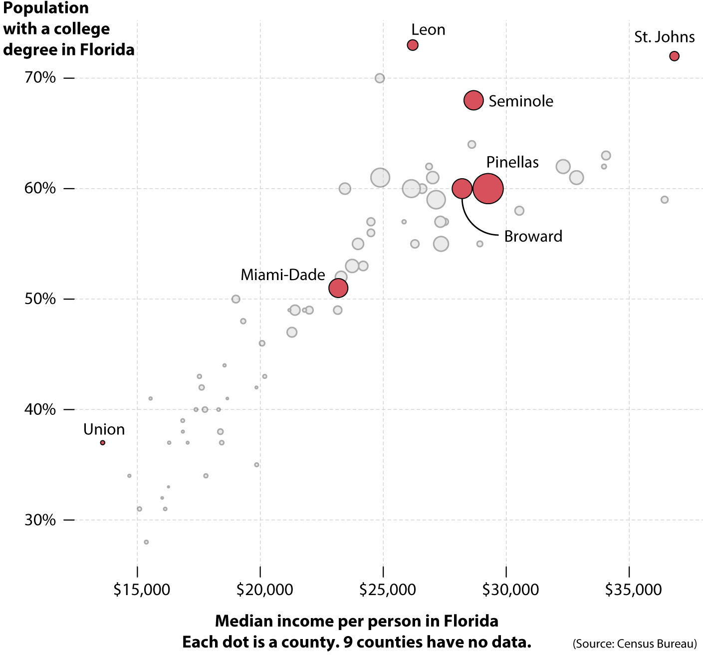
Here are some things I can perceive at a quick glance:
— In general, the higher the median income in a county (position on the horizontal axis), the higher the number of people who have a college education (position on the vertical axis). Income and education are positively associated.
— There are some exceptions to this pattern. For instance, Leon County, where the Florida state capital of Tallahassee is, has a very large percentage of college-educated people, but its median income isn’t that high. This may be due to many factors. For instance, it might be that Tallahassee has large pockets of poverty but also attracts very wealthy and highly educated individuals who want to work in government or to live close to the halls of power.
— Encoding population density with the area of the bubbles reveals that counties that are richer and have many college graduates tend to be more densely populated than those that are poorer.
In case you seldom read charts, you may be wondering how it’s possible to see so much so quickly. Reading charts is akin to reading text: the more you practice, the faster you’ll be able to extract insights from them.
That being said, there are several tricks that we can all use. First, always peek at scale labels, to determine what it is that the chart is measuring. Second, scatter plots have that name for a reason: they are intended to show the relative scattering of the dots, their dispersion or concentration in different regions of the chart. The dots on our chart are quite dispersed on both the horizontal and vertical scales, indicating that median county incomes vary a lot—there are very small and very large incomes—and the same applies to college education.
The third trick is to superimpose imaginary quadrants on the chart and then name them. If you do that, even if it’s just in your mind, you’ll immediately grasp that there aren’t any counties in the lower-right quadrant and few on the upper left. Most counties are in the top right (high income, high education) or the bottom left (low income, low education). You can see the result here:

A fourth trick is to trace an imaginary line that goes roughly through the center of the bubble cloud, which reveals the overall direction of the relationship between average income per person and percentage of people who have a college education. In this case, it’s a line pointing upward (I’ve erased the scale labels for clarity):2
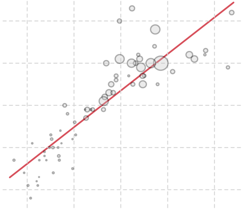
Once you apply these tricks, you’ll notice that the overall direction is right and up, meaning that the more you have of the metric on the horizontal axis (income), the more you have of the metric on the vertical one (college degrees). This is a positive association. Some associations are negative, as we saw in the introduction. For instance, income is negatively correlated with poverty rates. If we put poverty rates on the vertical (y) axis, our trend curve would go down, indicating that the higher the median income of a county, the lower its poverty rate will tend to be.
We should never infer from a chart like this that the association is causal. Statisticians like to repeat the mantra “Correlation doesn’t equal causation,” although associations are often the first step toward identifying causal connections between phenomena, given that you do enough inquiries. (I’ll have more to say about this in chapter 6.)
What statisticians mean is that we cannot claim from a chart alone that getting more college degrees leads to higher income, or vice versa. Those assertions may be right or wrong, or there may be other explanations for the high variation in median incomes and college education that our chart reveals. We just don’t know. Charts, when presented on their own, seldom offer definitive answers. They just help us discover intriguing features that may later lead us to look for those answers by other means. Good charts empower us to pose good questions.
Using area as a method of encoding is quite common in maps. In the introduction we saw several bubble maps displaying the number of votes received by each major candidate in the 2016 presidential race. Here’s another, with bubble area being proportional to population per county:
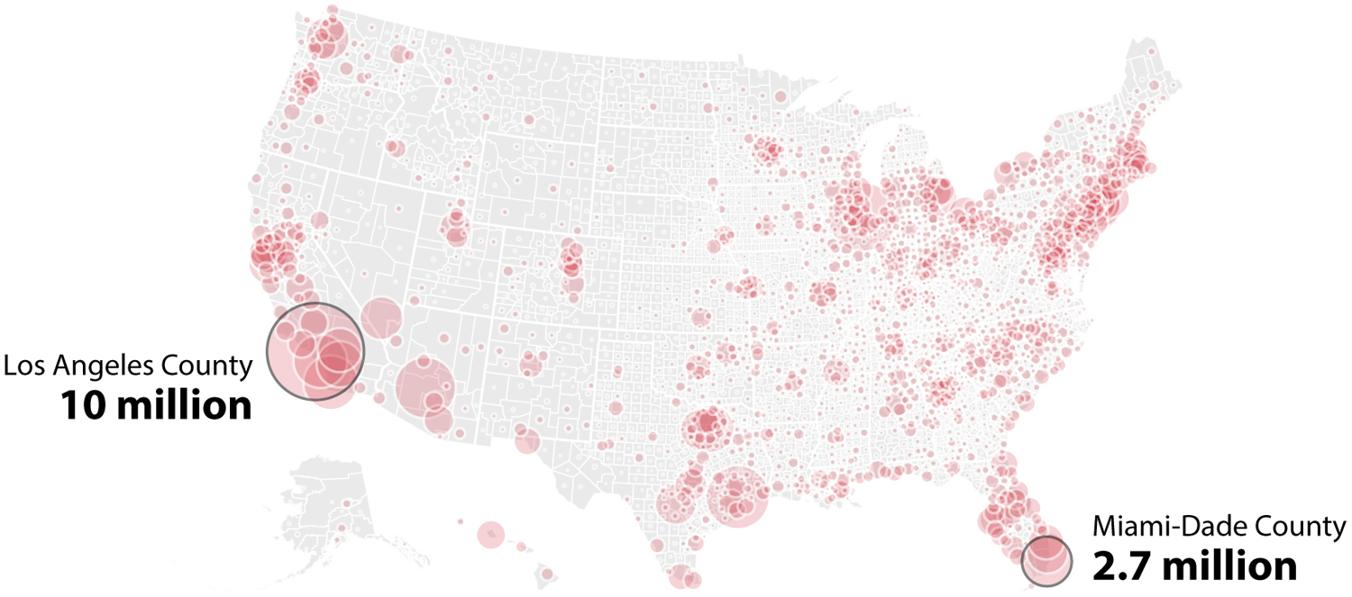
I highlighted Miami-Dade County because it’s where I live, and Los Angeles County because I didn’t know it was so massive. Los Angeles is the most populous county in the United States. It has nearly four times as many people as Miami-Dade. Let’s put the two bubbles side by side, and also encode the data with length, on a bar chart:
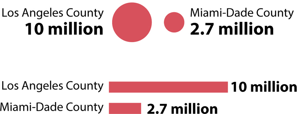
Notice that the difference between the sizes of the two counties looks less dramatic when population is encoded with area (bubble chart) than when it is encoded with length or height (bar chart).
Why does this happen? Think about it this way: A county of 10 million people has roughly four times the population of a county of 2.7 million people. If the objects we’re using are truly proportional to the numbers they are representing, we should be able to fit four bubbles the size of Miami-Dade’s into the bubble of Los Angeles, and four bars the length of Miami-Dade’s into Los Angeles’s bar. See for yourself (the smaller, black-outlined circles overlap, but their overlaps are similar in size to the empty spaces between them):
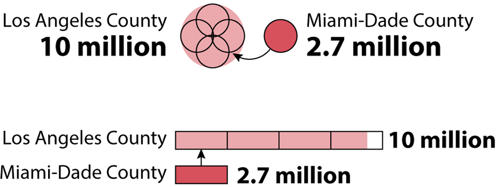
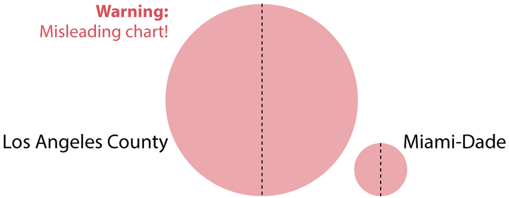
A very common mistake designers make when picking bubbles to represent data is to vary not their area but rather their height or length—their diameter—as if they were bar charts. It’s also a common trick used by those who want to exaggerate differences between numbers, so be warned.
Los Angeles has nearly 4 times the population of Miami-Dade, but if you quadruple the height of a circle, you’re also quadrupling its length. Thus, you aren’t making it 4 times its original size, but 16 times as big as it was before! See what happens if we scale the bubbles representing Los Angeles and Miami-Dade according to their diameter (wrong) and not their area (right). Now we can fit 16 bubbles the size of Miami-Dade’s inside Los Angeles’s bubble:
Many other kinds of charts use area as their method of encoding. For example, the treemap is increasingly favored in the news media. Paradoxically, it doesn’t look like a tree at all; instead, it looks like a puzzle made of rectangles of varying sizes. Here’s an example:
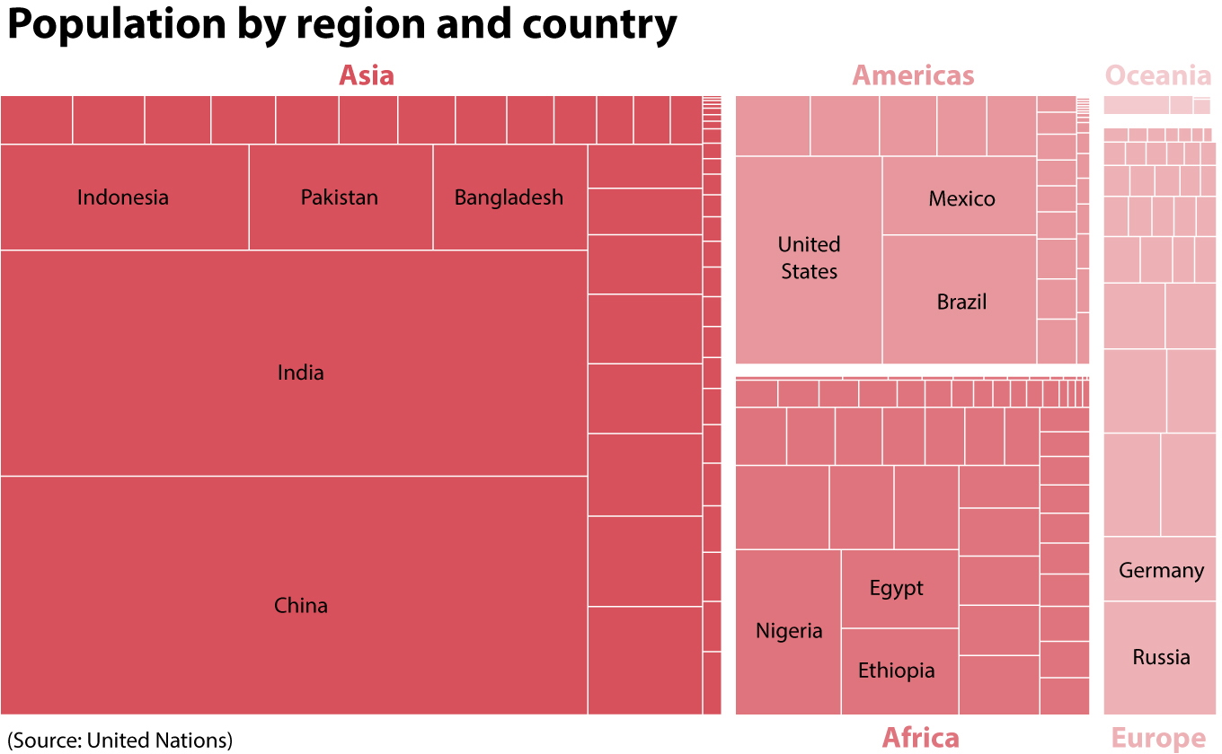
Treemaps receive their name because they present nested hierarchies.3 In my chart, each rectangle’s area is proportional to the population of a country. The combined area of the rectangles in a continent is also proportional to the population of that continent.
The treemap is sometimes used as a substitute for a more familiar graphic also based on area: the pie chart. Here’s one with the same continent population data above:
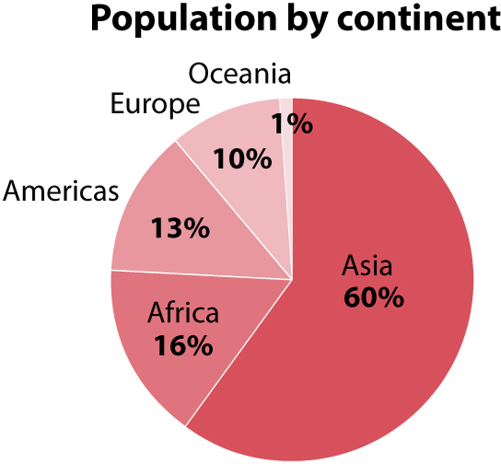
The area of the segments in a pie chart is proportional to the data, but so are its angles (angle is another method of encoding) and the arcs of each segment along the circumference. Here’s how it works: The circumference of a circle is 360 degrees. Asia represents 60% of the world population. Sixty percent of 360 is 216. Therefore, the angle formed by the two boundaries of the Asia segment needs to be 216 degrees.
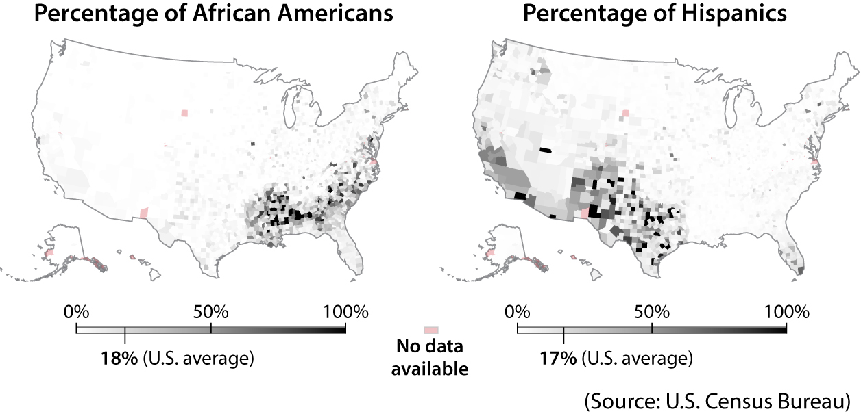
There are many other methods of encoding besides length/height, position, area, and angle. Color is among the most popular. This book begins with a map that employs both color hue and color shade: hue (red/gray) to represent which candidate won in each county, and shade (lighter/darker) to represent the winning candidate’s percentage of the vote.
These two maps show the percentage of African Americans and Hispanics per U.S. county. The darker the shade of grey, the larger the percentage of the population in these counties that is either African American or Hispanic:
Color shades are sometimes used to great effect in a kind of chart we can call a table heat map. In the following chart, the intensity of red is proportional to the variation of global temperatures in degrees Celsius per month and year in comparison to the average temperature of the 1951–1980 period:
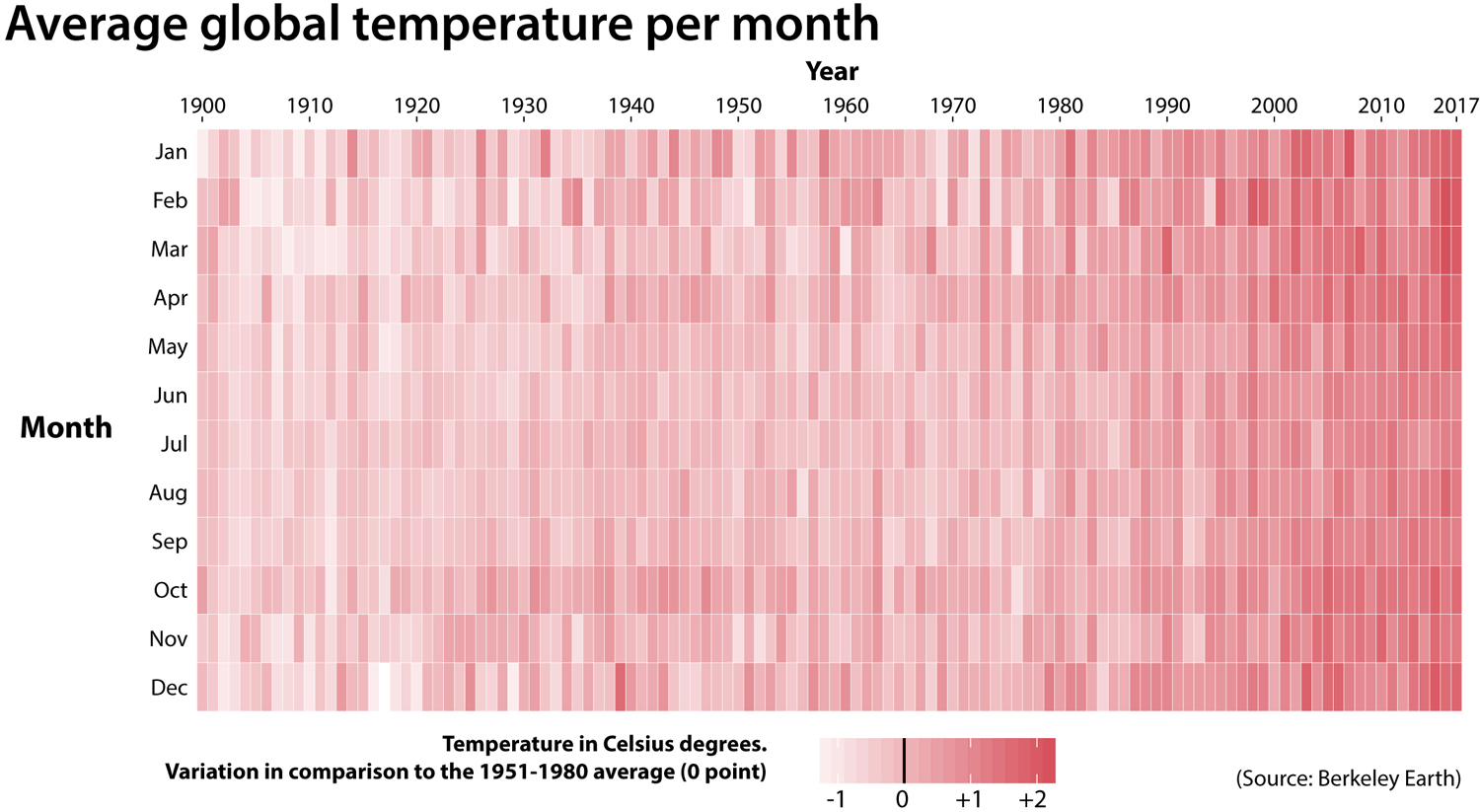
Each column of rectangles is a year, and each row is a month. The scale of a heat map isn’t as precise and detailed as others we’ve seen because the goal of this chart isn’t to focus on the specifics but on the overall change: the closer we get to the present, the hotter most months have become.
There are other ways of encoding data that are a bit less common. For instance, instead of varying the position, length, or height of objects, we could change their width or thickness, as on this chart, designed by Lázaro Gamio for the website Axios. Line width is proportional to the number of people or organizations that President Trump criticized on social media between January 20 and October 11, 2017:4

To summarize, most charts encode data through the variation of properties of symbols such as lines, rectangles, or circles. These properties are the methods of encoding we’ve just learned: the height or length, the position, the size or area, the angle, the color hue or shade, and so forth. We also learned that a chart can combine multiple methods of encoding.
Now, let me put you to the test. The following chart represents the fertility rates of Spain and Sweden between 1950 and 2005. Fertility rate is the average number of children per woman in a country. As you can see, in the 1950s, Spanish women had, on average, more children than did Swedish women, but the situation reversed in the 1980s. Try to identify what method or methods of encoding are at work here:
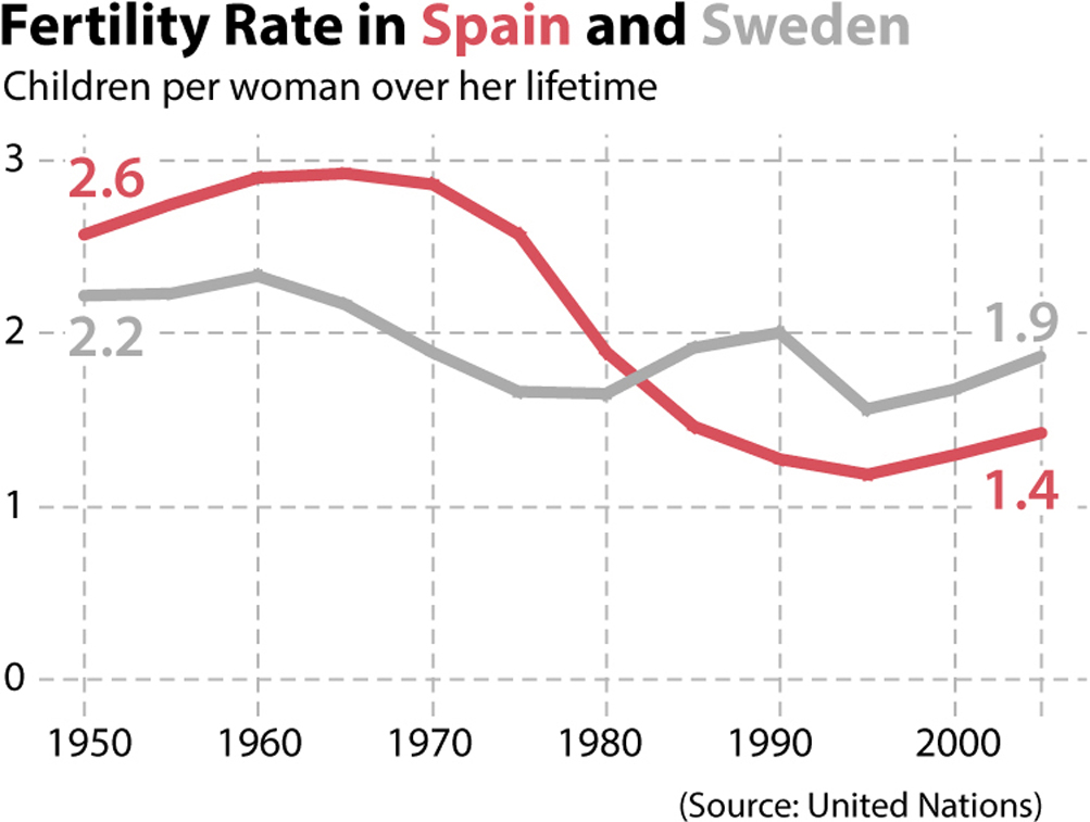
The first one is color hue, which is used to identify the two countries, Spain (red) and Sweden (grey).
The quantity itself, number of children per woman, is primarily encoded through position. Line graphs are created by placing dots on the horizontal axis—years, in this case—and on the vertical axis, in correspondence to the magnitude we’re measuring, and then connecting them with lines. If I eliminate the lines, the result is still a graphic showing the variation of the fertility rates in Spain and Sweden, although it’s a bit less clear:
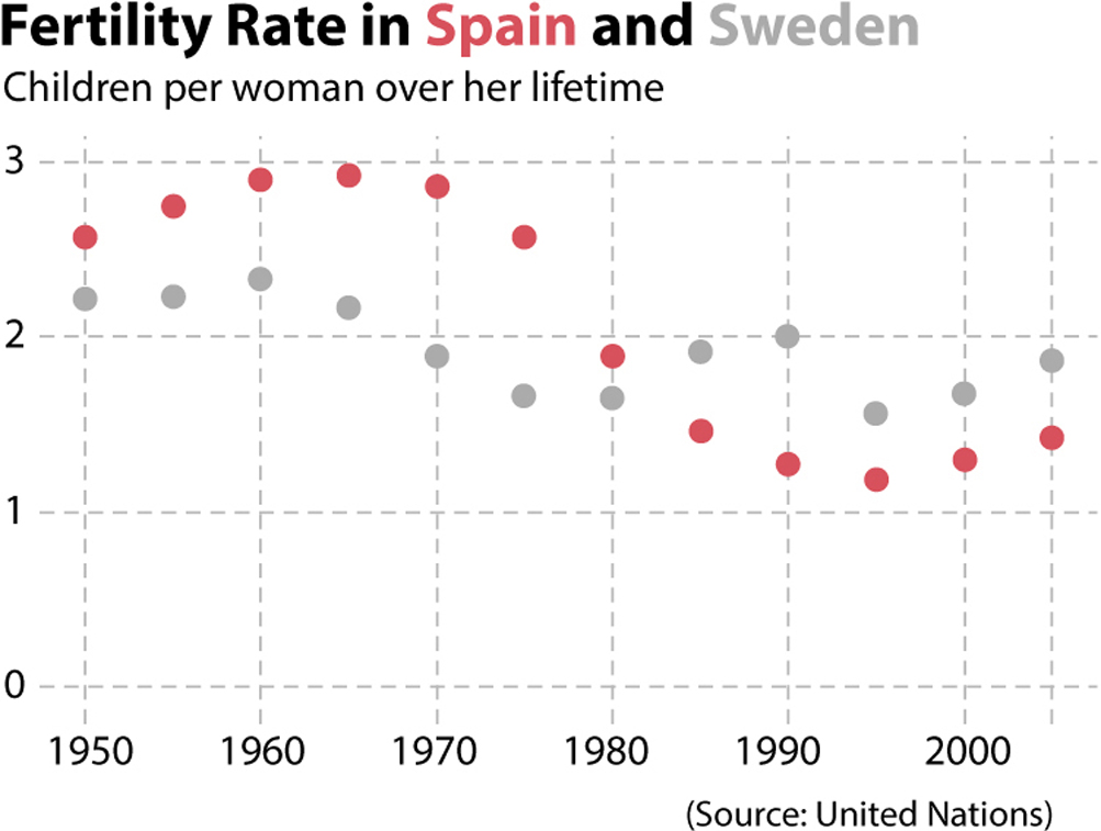
The slope also conveys information in a line graph, because when we connect the dots with lines, their slopes are a good indication of how steep or flat the variation is.
What about this chart? What are the methods of encoding here?

The first one you probably noticed is color shade: the darker the color of a country, the higher its gross domestic product per person. The second is area: those bubbles represent the populations of metropolitan regions that have more than one million people. That’s why, for instance, Miami isn’t on the map; the greater Miami area is a huge urban sprawl comprising several cities, none of them with more than one million inhabitants.
But there’s more. Position is also a method of encoding. Why? Think of what we learned at the beginning of this chapter: maps are constructed by locating points on a plane based on a horizontal scale (longitude) and a vertical scale (latitude). The landmasses and country borders on the map are made of many little dots connected to each other, and the positions of the city bubbles are also determined by the longitude and latitude of each city.
Cognitive psychologists who have written about how we read charts point out that our prior knowledge and expectations play a crucial role. They suggest that our brains store ideal “mental models” to which we compare the graphics we see. Psychologist Stephen Kosslyn has even come up with a “principle of appropriate knowledge”5 which, if applied to charts, means that effective communication between a designer (me) and an audience (you) requires that we share an understanding of what the chart is about and of the way data is encoded or symbolized in the chart. This means that we share roughly similar mental models of what to expect from that particular kind of chart.
Mental models save us a lot of time and effort. Imagine that your mental model of a line graph is this: “Time (days, months, years) is plotted on the horizontal axis, the amount is plotted on the vertical axis, and the data is represented through a line.” If that’s your mental model, you’ll be able to quickly decode a chart like this without paying much attention to its axis labels or title:

However, mental models can lead us astray. My own mental model of a line chart is much wider and more flexible than the one I described above. If the only mental model you have for a line chart is “time on the horizontal axis, magnitude on the vertical axis,” you’ll likely be confused by this graphic:
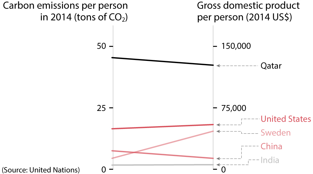
This is called a parallel coordinates plot. It’s also a chart that uses lines, but it doesn’t have time on the horizontal axis. Read the axis headers and you’ll see that there are two separate variables: carbon emissions per person; and gross domestic product, or GDP, per capita in U.S. dollars. The methods of encoding here, as in all charts that use lines to represent data, are position and slope: the higher up a country is on either scale, the bigger its carbon emissions or the wealth of its people.
Parallel coordinates plots were invented to compare different variables and see relationships between them. Focus on each country and on whether its line goes up or down. The lines of Qatar, the United States, and India are nearly flat, indicating that their position on one axis corresponds to the position on the other axis (high emissions are associated with high wealth).
Now focus on Sweden: people in Sweden contaminate relatively little, but their average per capita GDP is almost as high as that of U.S. citizens. Next, compare China and India: their GDPs per capita are much closer than their CO2 emissions per person. Why? I don’t know.6 A chart can’t always answer a question, but it’s an efficient way to discover intriguing facts that might ignite curiosity and cause you to pose better questions about data.
Here is another challenge. Now that you’re well into this chapter, you’ll have a pretty good mental model of a scatter plot. This one, in which I labeled some countries that I found curious, should be rather simple:
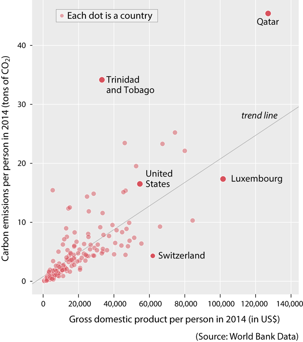
The mental model you have already developed for traditional scatter plots allows you to see that, with just some exceptions—some highlighted on the chart itself—the wealthier people in these countries are, the more they contaminate. But what if I show you another scatter plot, which looks like a line graph? You can see it on the next page.
Before your head explodes or you throw this book out the window, I should disclose that the first time I saw a chart like that, I was as befuddled as you. This type of chart, often called a connected scatter plot, is a bit hard to parse. Think about it this way:
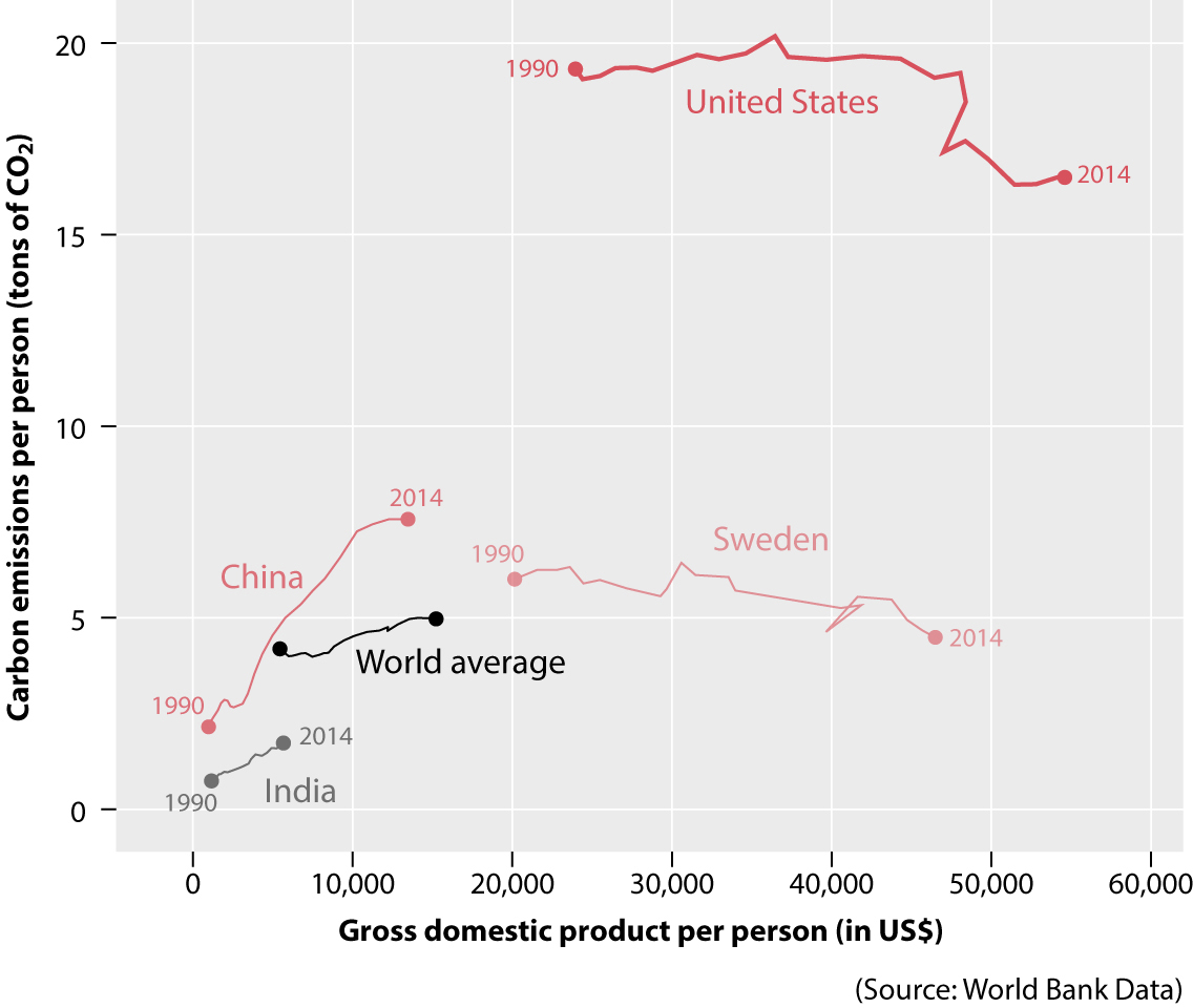
•Each line is a country. There are four country lines, plus a line for the world average.
•The lines are made by connecting dots, each corresponding to a year. I’ve highlighted and labeled only the first dot and the last dot on each line, corresponding to 1990 and 2014.
•The position of each dot on the horizontal axis is proportional to the GDP of the people in that country in that year.
•The position of each dot on the vertical axis is proportional to the amount of carbon emissions each person in those countries generated, on average, in that year.
The lines on this chart are like paths: they move forward or backward depending on whether people became richer or poorer, year by year, and they move up or down depending on whether people in those countries contaminated more or less. To make things clearer, let me add directional arrows to a couple of lines, plus a wind rose:
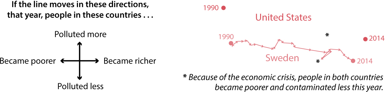
Why would anyone plot the data in such an odd way? Because of the point this chart is trying to make: at least in advanced economies, an increase in wealth doesn’t always lead to an increase in pollution. In the two rich countries I chose, the United States and Sweden, people became wealthier on average between 1990 and 2014—the horizontal distance between the two points is very wide—but they also contaminated less, such that the 1990 point is higher up than the 2014 point in both cases.
The relationship between GDP and pollution is often different in developing nations, because these countries usually have large industrial and agricultural sectors that contaminate more. In the two cases I chose, China and India, people have become wealthier—the 2014 point is farther to the right than the 1990 point—and, in parallel, they also contaminate much more. As you can see if you go back to the previous chart, the 2014 point is much higher than the 1990 one.
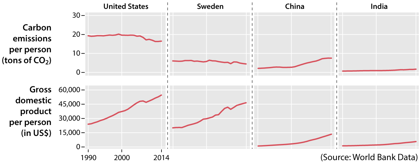
You may be thinking—and I’d agree—that to convey this message, it would also be appropriate to show the two variables, CO2 emissions and GDP per capita, as paired line graphs like the ones below.
Charts like the connected scatter plot are the reason why I began this chapter with the reminder that charts are seldom intuitive or self-explanatory, as many people believe. To read a chart correctly—or to create a good mental model of a type of chart we’ve never seen before—we must pay attention to it and never take anything for granted. Charts are based on a grammar and a vocabulary made of symbols (lines, circles, bars), visual encodings (length, position, area, color, and so on), and text (the annotation layer). This makes charting as flexible as using written language, if not more.
To explain something in writing, we assemble words into sentences, sentences into paragraphs, paragraphs into sections or chapters, and so on. The order of words in a sentence depends on a series of syntactic rules, but it may vary depending on what we want to communicate and on the emotional effect we want to instill. This is the opening of Gabriel García Márquez’s masterpiece, One Hundred Years of Solitude:
Many years later, as he faced the firing squad, Colonel Aureliano Buendía was to remember that distant afternoon when his father took him to discover ice.
I could convey the same information by assembling the words in a different manner:
Colonel Aureliano Buendía remembered the distant afternoon when his father took him to discover ice while facing the firing squad many years later.
The former opening has a certain musicality, while the latter is clunky and undistinguished. But both convey the same amount of information because they follow the same rules. If we read them slowly and carefully, we’ll grasp their content equally well, although we’ll enjoy the former more than the latter. Something similar happens with charts: if you just skim them, you won’t understand them—although you may believe you do—and well-designed charts aren’t just informative but also graceful and, like a good turn of phrase, sometimes even playful and surprising.
The same way that a long, deep, and complex sentence like that above can’t be understood in the blink of an eye, charts that display rich and worthwhile information will often demand some work from you. A good chart isn’t an illustration but a visual argument or part of an argument. How should you follow it? By taking the steps inside the red boxes I added to the following complex but illuminating chart by Washington Post data reporter David Byler.
1. Title, introduction (or caption), and source
If the chart includes a title and a description, read them first. If it mentions its source, take a look at it (more about this in chapter 3).
2. Measurements, units, scales, and legends
A chart must tell you what is being measured and how. Designers can do this textually or visually. Here, the vertical scale corresponds to the difference between the results of several special elections and the results of the 2016 U.S. presidential election. The horizontal scale is the number of days since Inauguration Day, January 20, 2017. The color legend tells us that the circles indicate who won each special election.
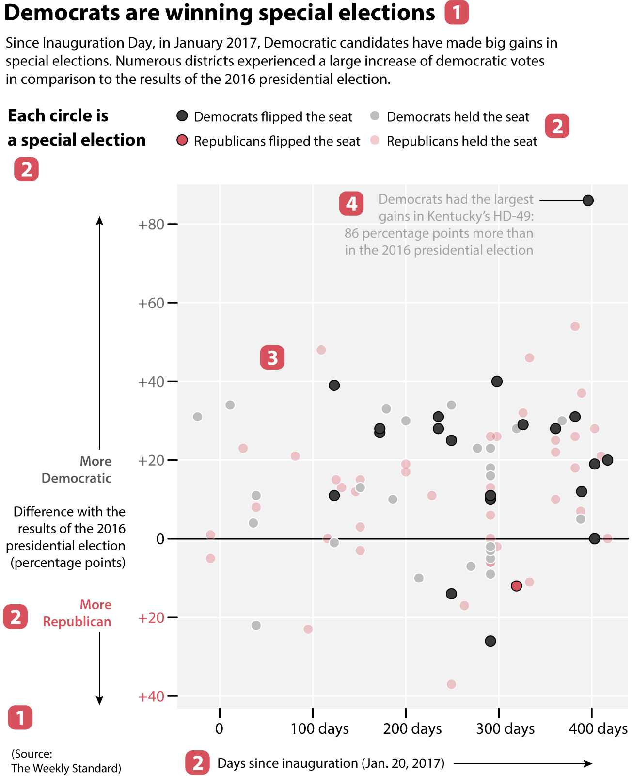
3. Methods of visual encoding
We’ve already spotted one: color. Grey indicates a Democratic victory; and red, a Republican victory. The color shade, darker or lighter, corresponds to whether either party flipped the seat.
The second method of encoding is position: position on the vertical axis is proportional to the difference in percentage points in comparison to the results of the 2016 presidential election. In other words, the higher above the zero baseline a circle is, the better Democrats did in comparison to 2016; the opposite is true if a circle is below the baseline.
To be even clearer: Imagine that in one of these districts Republicans got 60% of the vote in the 2016 presidential election and that, on this chart, this district’s circle sits on the +20 line above the baseline. This means that Republicans got just 40% of the vote in the current special election—that is, a +20 percentage point change in favor of Democrats (if there weren’t third-party candidates, of course).
4. Read annotations
Sometimes designers add short textual explanations to charts to emphasize the main takeaways or highlight the most relevant points. In this chart, you can see a note about a race in Kentucky’s House District 49, where the Democrats flipped the seat after getting a whopping 86 percentage point increase in support.
5. Take a bird’s-eye view to spot patterns, trends, and relationships
Once you have figured out the mechanics of a complex chart like this, it’s time to zoom out and think of patterns, trends, or relationships the chart may be revealing. When taking this bird’s-eye view, we stop focusing on individual symbols—circles, in this case—and instead try to see them as clusters. Here are a few facts I perceived:
•Since January 20, 2017, Democrats flipped many more seats from Republicans than Republicans from Democrats. In fact, Republicans flipped just one seat.
•In spite of that, both Democrats and Republicans held on to many seats.
•There are many more dots above the zero baseline than below it. This means that Democrats made big gains in the first 400 days after Inauguration Day, in comparison to their results in the 2016 presidential election.
How long did it take me to see all that? Much longer than you may think. Nevertheless, this is not a sign of a poorly constructed chart.
Many of us learned in school that all charts must be amenable to being decoded at a quick glance, but this is often unrealistic. Some elementary graphs and maps are indeed quick to read, but many others, particularly those that contain rich and deep messages, may require time and effort, which will pay off if the chart is well designed. Many charts can’t be simple because the stories they tell aren’t simple. What we readers can ask designers, though, is that they don’t make charts more complicated than they should be for no good reason.
In any case, and to continue with the analogy between charts and text I began a few pages back: you can’t assume you’ll interpret a news story or an essay well if you read its title alone or if you browse it inattentively or hastily. To extract meaning from an essay, you must read it from beginning to end. Charts are the same. If you want to get the most from them, you need to take a deep dive.
Now that we know how to read charts at a symbolic and grammatical level, defending ourselves against faulty ones becomes easier, and we can move to the semantic level of how to interpret them correctly. A chart may lie because:
•It’s poorly designed.
•It uses the wrong data.
•It shows an inappropriate amount of data—either too little or too much.
•It conceals or confuses uncertainty.
•It suggests misleading patterns.
•It panders to our expectations or prejudices.
If charts are based on representing data through different methods of encoding as faithfully as possible, then it won’t be surprising if I tell you that breaking this core principle will invariably lead to visual lies. We turn to them now.