Two is company, three is trumpery.
Jane G. Austin
Betty Alden: The First-born Daughter of the Pilgrims, 1891, p. 171.
In the previous chapter, we introduced the CCD—the first choice for practitioners of RSM because of its flexibility. As illustrated by a case study, an experimenter can hedge on RSM by adding CPs to a simpler, more economical two-level factorial. If curvature is not significant, it’s time to move on: why bother doing RSM if the surface is planar? On the other hand, if you detect a significant increase or decrease in response at the CP and it merits further attention, you can complete the CCD by adding the second block of axial points, including more CPs to provide a link with block one.
MUCH ADO ABOUT NOTHING?
In the previous chapters, we detailed a study on a reaction process that revealed a significant curvature effect of about 6 grams above the expected level of 82 grams. The chemist evidently felt that this deviation was too important to ignore, so the second block of the CCD was completed in order to construct a proper map of the nonlinear response. If the curvature had been overlooked despite being statistically significant, it would’ve made no difference in the end, because the same optimum emerges from the factorial model as that produced by the full CCD: low time, high temperature, and high rate. Thus, we get into an issue of statistical significance versus practical importance. Highly controlled automated assay optimization equipment now can accommodate DOEs with hundreds of reactions run at varying times, temperatures, plus other process factors and changing chemical compositions (Erbach et al., 2004). These massive designs have the statistical power to reveal tiny effects—some so small that they are of no practical importance. If you see the word significant trumpeted in technical reports, don’t be misled into thinking the research must then be considered important. Look at the actual effects generated by the experiment in relation to what should be considered of economic or other value.
Let every eye negotiate for itself and trust no agent; for beauty is a witch against whose charms faith melteth in blood.
Shakespeare
Much Ado about Nothing (II, i, 178–180)
The axial (star) points ideally (according to the developers Box and Wilson) go outside of the factorial box. This has advantages and disadvantages. It’s good to go further out for assessing curvature. However, it may be inconvenient for the experimenter to hit the five levels required of each factor: low axial (star at smallest value), low factorial, CP, high factorial, and high axial (star at greatest value). Furthermore, the stars may break the envelope of what’s safe or even physically possible. For example, what if you include a factor such as a dimension or a percent and the lower star point comes out negative? In such cases, the experimenter may opt to do a facecentered CCD (FCD) as shown in Figure 4.2.
Now let’s suppose you are confident that a two-level factorial design will not get the job done because you’re already in the peak region for one or more of the key process responses. The obvious step is upgrading to a three-level factorial (3k). However, as discussed in Chapter 3, though this would be a good choice if you’ve narrowed the field to just two key factors, beyond that the 3k becomes wasteful. Fortunately for us, George Box put his mind to this and with assistance from Box and Behnken (1960) came up with a more efficient three-level design option.
FEELING LUCKY? IF SO, CONSIDER A “DEFINITIVE SCREENING DESIGN”
In the third edition of DOE Simplified, we introduce definitive screening designs (DSDs) as near-minimal run (2K + 1) resolution IV templates for uncovering main effects, their novelty being a layout with three (not just two) levels of each factor (Jones and Nachtsheim, 2011). Because DSDs generate squared terms, they serve as a response surface method. However, you must have at hand the right computational tools for deriving a model from a design with fewer runs than the number of coefficients in the model, that is, a “supersaturated” experiment.
This not being a robust choice for an RSM design, we recommend you take the DSD short cut only under extenuating circumstances. If you do, apply forward selection (mentioned in Chapter 2’s side note “A Brief Word on Algorithmic Model Reduction”) using the Akaike (pronounced ah-kahee-keh) information criterion (AICc), rather than the usual p values. The small “c” in the acronym refers to a correction that comes into play with small samples to prevent overfitting.
An easygoing overview on AICc is provided by Snipes and Taylor in a case study (2014) applying this criterion to the question of whether the more you pay for wine the better it gets. For reasons which will become apparent, consider pouring yourself a chilled Chardonnay before downloading this freely available (under a Creative Commons license) publication from www.sciencedirect.com/science/article/pii/S2212977414000064.
BBDs are constructed by first combining two-level factorial designs with incomplete block designs (IBD) and then adding a specified number of replicated CPs.
INCOMPLETE BLOCK DESIGNS
An IBD contains more treatments than can be tested in any given block. This problem emerged very early in the development of DOE for agricultural purposes. For example, perhaps only two out of three varieties of a crop could be planted at low and high levels in any of three possible fields. In such a case, any given field literally represented a block of land within which only an incomplete number of crop varieties could be tested. Incomplete blocks may occur in nonagricultural applications as well. Let’s say you want to compare eight brands of spark plugs on a series of six-cylindered engines in an automotive test facility. Obviously, one engine block can only accommodate an incomplete number of plugs (six out of the eight).
Table 5.1 Component Elements of Three-Factor BBD
a |
b |
A |
B |
C |
|
−1 |
−1 |
a |
b |
0 |
|
+1 |
−1 |
a |
0 |
b |
|
−1 |
+1 |
0 |
a |
b |
|
+1 |
+1 |
0 |
0 |
0 |
Table 5.1 provides the elements for building a three-factor BBD. On the left, you see a two-level factorial for two factors: a and b. Wherever these letters appear in the incomplete block structure at the right, you plug in the associated columns to create a matrix made up of plus 1s (high), minus 1s (low), and 0s (center).
So, for example, the first run in standard order is −1, −1, 0. Then comes +1, −1, 0, and so forth, with +1, +1, 0 being the last of the first group of four runs. The following four runs will all be set up with B at the 0 level. After four more runs with A at zero the design ends with a CP—all factors being at the zero level. At least three CP runs are recommended for the BBD (Myers et al., 2016, p. 413). However, we advise starting with five and going up from there for designs with more factors. Table 5.2 shows the end result: 17 runs including five replicated CPs.
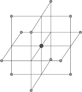
Figure 5.1 shows the geometry for this three-factor BBD, which displays 12 edge points lying on a sphere about the center (in this case at √2) with five replicates of the CP.
The 13 unique combinations represent less than one-half of all possible combinations for three factors at three levels (33 = 3 * 3 * 3 = 27) and yet they provide sufficient information to fit the 10 coefficients of the quadratic polynomial.
LESSON ON GEOMETRY FOR BBD
Although the description is accurate for three factors, it is misleading to refer to edge points as a geometric element. That’s why our picture lays out the points as corners of squares (consistent with the incomplete block structure). The BBD uses only −1, 0, and +1 for the factor levels, so the design points are actually the centroids of the (k − m) dimensional faces of the k-dimensional cube, where m is the number of ±1’s in a design row and k represents the number of factors. For the special case of the three-factor BBD, k is 3 and m is 2, so the design points fall on the center of the one (k − m = 3 − 2 = 1) dimensional faces—that is, the centers of the cubical edges.
BBDs are geared to fit second-order response surfaces for three or more factors. The BBDs are rotatable (for k = 4, 7) or nearly so. Table 5.3 shows how many runs, including CPs, are needed as a function of the number of factors up to seven.
As shown above, most BBDs can be safely subdivided into smaller blocks of runs. Templates for these designs and for many more factors are available via the Internet (Block and Mee) and encoded in RSM software (Design-Expert, Stat-Ease, Inc.). Bigger and bigger BBDs, accommodating 20 or more factors, are currently being developed by the statistical academia (Mee, 2003).
Std |
A |
B |
C |
1 |
−1 |
−1 |
0 |
2 |
+1 |
−1 |
0 |
3 |
−1 |
+1 |
0 |
4 |
+1 |
+1 |
0 |
5 |
−1 |
0 |
−1 |
6 |
+1 |
0 |
−1 |
7 |
−1 |
0 |
+1 |
8 |
+1 |
0 |
+1 |
9 |
0 |
−1 |
−1 |
10 |
0 |
+1 |
−1 |
11 |
0 |
−1 |
+1 |
12 |
0 |
+1 |
+1 |
13 |
0 |
0 |
0 |
14 |
0 |
0 |
0 |
15 |
0 |
0 |
0 |
16 |
0 |
0 |
0 |
17 |
0 |
0 |
0 |
Figure 5.1 Layout of points in a three-factor BBD.
Factors k |
BBD Runs (CPs) |
BBD Blocks |
3 |
17 (5) |
1 |
4 |
29 (5) |
1 or 3 |
5 |
46 (6) |
1 or 2 |
6 |
54 (6) |
1 or 2 |
7 |
62 (6) |
1 or 2 |
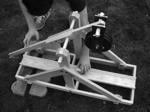
The following case study makes use of a scale-model trebuchet built by the South Dakota School of Mines and Technology (SDSMT) for experimentation by their engineering students. Figure 5.2 shows it being made ready to fire a rubber racquetball.
The ball is held in a sling attached to a wooden arm via fishing line. When the arm is released by the trebuchet operator, the counterweights lever it upward—causing the ball to be flung forward 100 feet or more. Notice the holes drilled through the wooden arm, which allow various configurations for placement of the weights and the pivot point. Here’s what we studied:
Figure 5.2 SDSMT trebuchet.
A. Arm length: 4–8 inches (in.) from counterweight end to pin that held weights
B. Counterweight: 10–20 pounds (lbs)
C. Missile weight: 2–3 ounce (oz.) racquetball filled with varying amounts of salt
QUICK PRIMER ON MEDIEVAL MISSILE-HURLING MACHINERY
Catapults, energized by tension or torsion, may be more familiar to you than the trebuchet (pronounced “treb-you-shay”), which uses a counterweight. The first trebuchets were built prior to the fifth century b.c. in China (Chevedden, 1995). The technology migrated to Europe where machines like this used for war became known as engines (from the Latin ingenium or ingenious contrivance). Operators of trebuchets were called “ingeniators”—a precursor to a profession now known as engineering. Britain’s King Edward, villainously depicted in the movie Braveheart, kept a whole crew of ingeniators busy bombarding the Scottish-held Stirling Castle in 1304 with 13 trebuchets going day and night. They saved their biggest engine of war, called the “War Wolf,” for the coup de grâce—firing several missiles despite efforts by the Scots to surrender first. Trebuchets used a variety of ammunition, mainly stone balls, but also beehives, barrels of pitch or oil that could be set ablaze, animal carcasses to spread diseases, and hapless spies—captured and repatriated as the crow flies.
A heavy silence descended … I stepped back to contemplate “the beast.” She was truly magnificent—powerful, balanced, of noble breed.
Renaud Beffeyte
An ingeniator for trebuchets reproduced at Loch Ness, Scotland, for a public television show by NOVA (Hadingham, 2000)
These three key factors were selected based on screening studies performed by SDSMT students (Burris et al., 2002). The experiments were performed by one of the authors (Mark) and his son (Hank) in the backyard of their home. To make the exercise more realistic, they aimed the missiles at an elevated play fort about 75 feet from the trebuchet. It took only a few pre-experimental runs to determine what setting would get the shots in range of the target. At first, the ingeniators (see sidebar titled “Quick Primer on Medieval Missile-Hurling Machinery” for explanation of term) tried heavier juggling balls (1–2.5 pounds), but, much to their chagrin, these flew backward out of the sling. The lighter racquetballs worked much better—flying well beyond 75 feet over the fence and into the street. (Beware to neighbors strolling with their babies by the Anderson household!)
Based on the prior experiments and physics (see the “Physics of the Trebuchet” note), it made no sense to simply do a two-level factorial design: RSM would be needed to properly model the response. It would have been very inconvenient to perform a standard CCD requiring five-factor levels. Instead, the experimenters chose the BBD specified in Table 5.2. The ranges for arm length (factor A) and counterweight (B) were chosen to be amenable with the SDSMT trebuchet. These factors were treated as if they could be adjusted to any numerical level, even though in practice this might require rebuilding a trebuchet to the specified design.
PHYSICS OF THE TREBUCHET
The trebuchet is similar to a first-order lever, such as see-saws or teeter-totters you see at the local playgrounds. Force is applied to one end, the load is on the other end, and the fulcrum sits between the two. Imagine putting a mouse on one end of the see-saw and dropping an elephant on the other end—this illustrates the physics underlying the trebuchet. These principles were refined for centuries by ancient war-mongers. For example, in the fourteenth century, Marinus Sanudus advised a 1:6 ratio for the length of the throwing arm to the length of the counterweight arm, both measured from the point of the fulcrum (Hansen, 1992). Arabic sources suggested that to get maximum effect from basketfuls of poisonous snakes, the length of the sling should be proportional to the length of the throwing arm. Physics experts can agree on the impact of these variations in length because their effects on leverage are well known. However, they seem to be somewhat uncertain about other aspects of trebuchet design, such as
 Adding wheels to the base (evidently helps by allowing weight to drop more vertically as the trebuchet rolls forward in reaction to release)
Hinging the weight rather than fixing it to arm (apparently this adds an extra kick to the missile)
The results from the 17-run BBD on the SDSMT trebuchet are shown in Table 5.4. The response (y) was distance measured in feet.
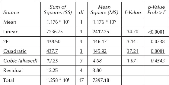
Standard order 9 (run number 14) actually hit the elevated fort, so the short distance it would have traveled beyond that was estimated at 8 feet (so total = 75 + 8 = 83). Notice from the last five runs in standard order, all done at CP levels, how precisely the trebuchet threw the racquetball. Because it was tricky to get an exact spotting for landings, the measurements were rounded to the nearest foot, so the three results at 91 actually varied by a number of inches, but that isn’t much at such a distance. The relatively small process variation, in comparison to the changes induced by the controlled factors, led to highly significant effects. You can see this in the sequential model sums of squares statistics in Table 5.5.
Table 5.4 Results from Trebuchet Experiment (Underlined Shot Hit the Target)
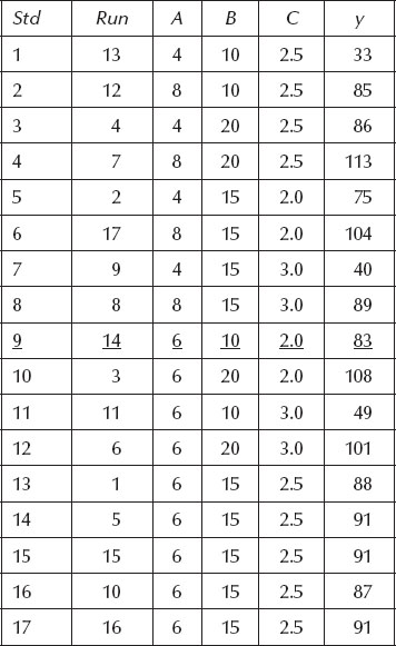
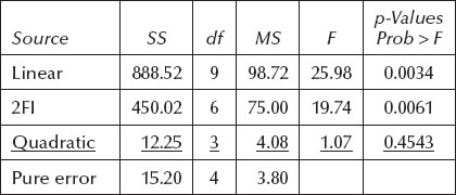
Table 5.5 Sequential Model Sums of Squares
HOLLYWOOD TAKES ON THE TREBUCHET
To get a look at a trebuchet in action, rent or stream the video for The Last Castle (2001) starring Robert Redford (the hero, naturally) and James Gandolfini as a sadistic warden. Be forewarned that this movie, like many produced in Hollywood, features a number of highly improbable occurrences, which could only happen in an alternate universe in which the laws of physics, probability, and common sense no longer apply. For example, Redford supervises construction of a collapsible trebuchet under the noses of the guards, using only the materials available in the prison workshop and then trains his crew to use it during exercise breaks, so when the climactic riot occurs, they can then fling a rock through the warden’s window for a direct hit on to his prized display case of weaponry. According to one reviewer (Andrew Howe, FilmWritten, November 20, 2001. http://www.efilmcritic.com/review.php?movie=5566&reviewer=193), The Last Castle is “a jaw-dropping, bone-crunching mess of a film, the product of one too many mind-altering substances.” However, it’s very inspiring if you aspire to be a master ingeniator with a trebuchet.
Table 5.5 shows that linear terms significantly improve the fit over simply taking the mean of all responses. The 2FI terms appear to fall into the gray area between p of 0.05 and 0.10, but be careful. These probability values are biased due to an error term that contains variability, which will be explained by the next order of terms. We talked about this in a note titled “Necessary, But Not Sufficient” in the previous chapter. Be sure to look again at these 2FI terms at the ANOVA stage of the analysis. There’s no doubt about the quadratic terms—they are highly significant (p of 0.0001). The BBD does not support estimation of all cubic terms so this model is aliased and shouldn’t be applied.
The quadratic model appears to adequately represent the actual response surface based on its insignificant lack of fit (p >> 0.1) shown in Table 5.6.
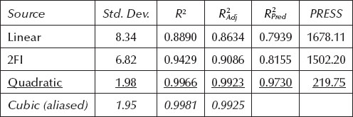
Overall, the quadratic model emerges best according to the model summary statistics listed in Table 5.7.
Table 5.8 displays the ANOVA for the full quadratic model.
All quadratic terms except for B2 achieve significance at the 0.05 p-value threshold (95% CI). We will carry this one insignificant term along with the rest. The residuals from this full quadratic model exhibit no aberrant patterns on the diagnostic plots discussed in previous chapters (normal plot of residuals, residuals versus predicted level, etc.), so we now report the results.
Table 5.7 Model Summary Statistics

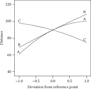
Before generating the more interesting 2D contour and 3D response surfaces, it will be helpful to take a simplistic view of how the three control factors affected the distance off the trebuchet. This can be seen on the perturbation plot shown in Figure 5.3.
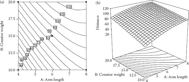
As you can infer from B2 not being significant according to ANOVA, the track for factor B exhibits no curvature (nonlinearity). On the other hand, factor A exhibits a noticeable bend. Factor C exhibits only a very slight curve. Only two of these three factors can be included on contour and 3D plots. Obviously, A should be one of them because it’s the most arresting visually. Figure 5.4a and b shows the contour plot and corresponding 3D view for A (arm length) versus B (counterweight) while holding C (missile weight) at its CP value (2.5 ounces).
Figure 5.3 Perturbation plot.
Figure 5.4 (a) 2D plots (C centered). (b) 3D plot (C centered).
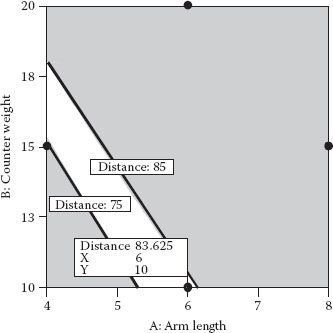
Figure 5.5 Graphical overlay plot (factor C constant at low level).
Notice on the 2D plot in Figure 5.4a how the contours for 75–85 feet pass diagonally roughly through the middle. This range represents the operating window or sweet spot. It puts the 2.5-ounce missile somewhere on the target at a broad array of A–B setup combinations.
The graphical overlay plot shown in Figure 5.5 provides a compelling view of the sweet spot at a different slice for factor C—its lower level (2.0-ounce missile).
The flag shows the setup used at standard order 9 listed on Table 5.4, which actually hit the fort as predicted.
WHAT TO DO WHEN AN UNEXPECTED VARIABLE BLOWS YOU OFF COURSE
The trebuchet experiment was done outdoors under ideal conditions—calm and dry. In other circumstances, the wind could have built up to a point where it affected the flight of the missile. Ideally, experimenters confronted with environmental variables like this will have instruments that can measure them. For example, if you know that temperature and humidity affect your process, keep a log of their variations throughout the course of the experiment. In the case of the trebuchet, an anemometer would be handy for logging wind magnitude and direction. If you think such a variable should be accounted for, add it to the input matrix as a covariate. Then, its contribution to variance can be accounted for in the ANOVA, thus revealing controlled factors that might otherwise be obscured.
Hornblower told himself that a variation of two hundred yards in the fall of shot from a six pounder at full elevation was only to be expected and he knew it to be true, but that was cold comfort to him. The powder varied from charge to charge, the shots were never truly round, quite apart from the variations in atmospheric conditions and in the temperature of the gun. He set his teeth, aimed and fired again—short and a trifle to the left. It was maddening!
C.S. Forester
Flying Colours (1938)
PRACTICE PROBLEM
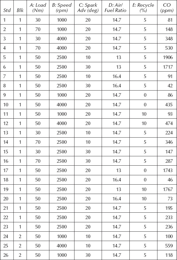
5.1 RSM experiments on gasoline engines help automotive companies predict fuel consumption, exhaust emissions, etc. as functions of engine rpm, load, and so on. The prediction equations then become the basis for managing engine parameters via on-board computers in cars. For example, Ford Motor Limited of the United Kingdom applied a BBD to maximize fuel (or as they call it, “petrol”) efficiency and minimize various exhaust emissions as a function of five key factors (Draper et al., 1994):
A. Engine load, Newton meters (N m): 30–70
B. Engine speed, revolutions per minute (rpm): 1000–4000
C. Spark advance, degrees (deg): 10–30
D. Air-to-fuel ratio: 13–16.4
E. Exhaust gas recycle, percent of combustion mixture (%): 0–10
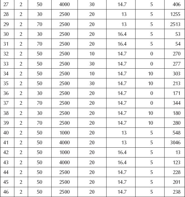
The automotive engineers divided this 46-run experiment into two blocks, presumably on two test engines. The results for one of the emissions, carbon monoxide (CO), are shown in Table 5.9. Obviously, this should be minimized.
Using the software associated with this book, you can set up this five-factor BBD and enter the results for the CO emissions. (Or save time by opening the file named “Prob 5-1 emissions.dx*” available via the Internet: see Appendix 5A on software installation for a path to the website offering files associated with the book.) After creating the design (or opening the file), we suggest you put it in standard order to enter the data (or look it over)—it will come up by default in random run order. Then, analyze the results.
Watch out for significant lack of fit and problems in the diagnostic plots for residuals, especially the Box–Cox plot (see Appendix 5A). Then, reanalyze the data with a log transformation (previously applied to the American football example in Chapter 2—and discussed in Appendix 2A). If you get bogged down on the transformations or any other aspect of this case, don’t belabor the problem: see what we’ve done in the solution (stored in Adobe’s PDF) posted at the same website where you found the data for this problem).
AUTOMOTIVE TERMINOLOGY IN THE UNITED KINGDOM VERSUS UNITED STATES
One of the authors (Mark) had a very pleasurable time driving a rented Ford (United Kingdom) Mondeo while traveling in Ireland. Upon returning to the United States, he learned that Ford sold the same car under the name “Contour,” which for an enthusiast of RSM could not be resisted—it was promptly purchased! More than just the brand names change when automotive technology hops over “The Pond” (Atlantic Ocean)—a whole set of terms must be translated from English to American English. For example, the original authors (UK-based) of the case described in Problem 5.1 refer to “petrol” rather than “gasoline,” as we in the United States call it. The UK affiliate for Stat-Ease once told a story about how he tracked down a problem in his vehicle, which required looking under the “bonnet” (hood) and checking the “boot” (trunk). His UK-made engine was made from “aluminium” (aluminum). It starts with power from the “accumulator” (battery), which is replenished by the “dynamo” (generator). An indicator for the battery and other engine aspects can be seen on the “fascia” (dashboard). Our man in the United Kingdom checks the air pressure in his “tyres” (tires) with a “gauge” (gage) and holds parts to be repaired in a “mole wrench” (vice grips) or, if it’s small enough, a “crocodile clip” (alligator clip). Repairs are done with the aid of a “spanner” (wrench), perhaps by the light of a “torch” (flashlight). When he heads down the “motorway” (highway) dodging “lorries” (trucks), the British driver’s engine sounds are dampened by the “silencer” (muffler).
We have everything in common with America nowadays, except, of course, the language.
Oscar Wilde
From his romantic comedy The Canterville Ghost, 1887
Giving English to an American is like giving sex to a child. He knows it’s important but he doesn’t know what to do with it.
Adam Cooper (nineteenth century)
Appendix 5A: Box–Cox Plot for Transformations
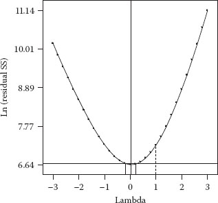
This is as good a time as any to introduce a very useful plot for response transformations called the “Box–Cox” (Box and Cox, 1964). You should make use of this plot when doing Problem 5.1. Figure 5.6 shows a Box–Cox plot for the regression analysis of quarterback (American football) sacks reported in Chapter 2. It was produced by applying a linear (first-order) model: ŷ = f (height, weight, years, games, and position).
The plot indicates the current power (symbolized mathematically by the Greek letter lambda) by the dotted line at 1 on the x-axis. This represents no transformation of the actual response data (y1). Alternatively, the response is transformed by a range of powers from −3 (inverse cubed) to +3 (cubed). The transformed data are then refitted with the proposed model (in this case linear) and the residual SS generated in a dimensionless scale for comparative purposes. (Box and Cox recommended plotting against the natural logarithm (ln) of the residual SS (versus the raw SSresidual), but this is not of critical importance.) The minimum model residual can then be found (see the tall line in plot) and the CI calculated via statistical formulas (displayed on either side of the minimum with short lines). In this case (football data), notice that the current point (the dotted line) falls outside of the 95% CI. Therefore, applying a different power, one within the CI at or near the minimum, will be advantageous. It’s convenient in this case to select a power of 0, which represents the logarithmic transformation, either natural or base 10—it does not matter: the difference amounts to only a constant factor (Box and Draper, p. 289).
Figure 5.6 Box–Cox plot for football data.
The indication for log transformation (lambda (λ) zero) given by the Box–Cox plot shown in Figure 5.6 is very typical of data that varies over such a broad range (18-fold in this case). However, this is just one member from a family of transformations—designated as power law by statisticians—you should consider for extreme response data. Other transformations that might be revealed by the Box–Cox plot are
Square root (0.5 power), which works well for counts, such as the number of blemishes per unit area
Inverse (−1 power), which often provides a better fit for rate data
George Box and his colleagues offer these general comments on transformations, in particular the inverse (Box et al., 1978, p. 240): “The possibility of transformation should always be kept in mind. Often there is nothing in particular to recommend the original metric in which the measurements happen to be taken. A research worker studying athletics may measure the time t in seconds that a subject takes to run 1000 meters, but he could equally well have considered 1000/t, which is the athlete’s speed in meters per second.”
THE POWER-LAW FAMILY
This might be a good description for a family of high-priced lawyers of several generations, such as “Smythe, Smythe, and Smythe, Attorneys-at-Law.” However, it’s something even more scary—a statistical description of how the true standard deviation (σ) might change as a function of the true mean (μ). Mathematically, this is expressed as
Ideally, there is no relationship (the exponent α equals 0), so no transformation is needed (lambda (λ) minus alpha (α) equals 1, so the power-law specifies y1, which leaves the responses in their original metric). When standard deviation increases directly as a function of the mean (α = 1), you may see a characteristic megaphone pattern (looks like: <) of residuals versus predicted response. In other words, the residuals increase directly as the level of response goes up. Then, it will be incorrect to assume that variance is a constant and thus can be pooled for the ANOVA. In such cases, the log transformation will be an effective remedy (because λ = 1 − α = 1 − 1 = 0 and y0 translates to ln(y)).
Other transformations, not part of the power-law family, may be better for certain types of data, such as applying the arc-sin square root to fractiondefect (proportion pass/fail) data from quality control records (see Anderson and Whitcomb, 2003, for details).
To summarize this and previous discussion on diagnosing needs for response transformation:
1. Examine the following residual plots (all studentized) to diagnose nonnormality (always do this!):
a. Normal plot
b. Residuals versus predicted (check on assumption of constant variance)
c. Externally studentized (outlier t) versus run number
d. Box–Cox plot (to look for power transformations)
2. Consider a response transformation as a remedy, such as
a. The logarithm (base 10 or natural, it does not matter)
b. Another one from the power-law family such as square root (for counts) or inverse (for rates)
c. Arc-sin square root (for fraction defects) and other functions not from the power-law family