Factorials to Set the Stage for More Glamorous RSM Designs
When you come to a fork in the road, take it.
Yogi Berra
Ask just about anyone how an experiment should be conducted and they will tell you to change only one factor at a time (OFAT) while holding everything else constant. Look at any elementary science text and you will almost certainly find graphs with curves showing a response as a function of a single factor. Therefore, it should not be surprising that many top-notch technical professionals experiment via OFAT done at three or more levels.
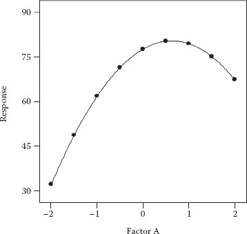
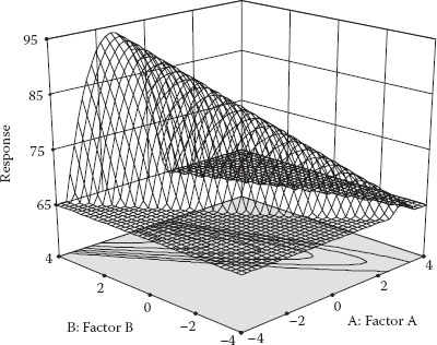
Does OFAT really get the job done for optimization? Let’s put this to the test via a simulation. Recall in Chapter 1 seeing a variety of response surfaces. We reproduced a common shape—a rising ridge—in Figure 3.1.
The predictive equation for this surface is
This will be our model for the following test of OFAT as an optimization method.
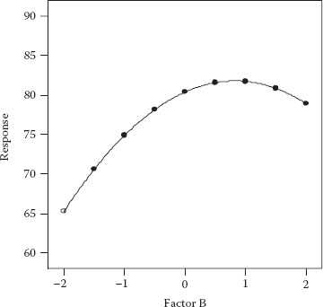
Assume that the OFAT experimenter arbitrarily starts with factor A and varies it systematically over nine levels from low to high (−2 to +2) while holding factor B at mid-level (0). The resulting response curve can be seen in Figure 3.2.
Figure 3.1 Rising ridge.
The experimenter sees that the response is maximized at an A-level near one (0.63 to be precise). The next step is then to vary B while holding factor A fixed at this “optimal” point. Figure 3.3 shows the results of the second OFAT experiment.
Figure 3.2 OFAT plot after experimenting on factor A.
Figure 3.3 OFAT plot for factor B (A fixed at 0.63).
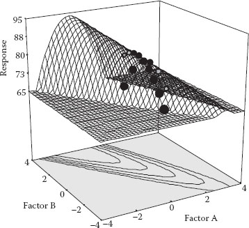
The response is now increased from 80 (previous maximum) to 82 by adjusting factor B to a level of 0.82 based on this second response plot. The OFAT experimenter proudly announces the optimum (A, B) combination of (0.63, 0.82), which produced a response above 80 in only 18 runs. However, as you can see in Figure 3.4, the real optimum is far higher (~94) than that attained via OFAT.
Figure 3.4 OFAT points shown on true surface.
By changing only one factor at a time, this experimenter got to the top of the ridge but did not realize that more could be gained by traveling up it. Furthermore, the results for the OFAT search on this surface will depend greatly on where B is fixed when A is varied and vice versa. A better DOE is needed to detect the interaction of AB that causes this unanticipated increase.
ADVICE FOR NINTH GRADERS ON EXPERIMENTATION
A science textbook used by ninth graders in the United States (Smith et al., 1993) advises that students vary only one condition while holding all others constant. They follow up with an activity that involves tying strings of varying length to two bolts, and hanging them from a string that also can differ in length. The students are asked to swing one of the bolts and record movement of the other (it’s a physics thing!). Then it’s suggested they change the weight of the bolt and see what happens. So, in the end, students experiment on many variables, but the follow-up question makes it clear how they should do it: “Why is it important to change only one variable at a time?” OFAT strikes again!
The present method of experiment is blind and stupid; hence men wandering and roaming without any determined course, and consulting mere chance, are hurried about to various points, and advance but little…
Francis Bacon
Novum Organum, First Book, 70 (1620)
Factorial Designs as an Option to OFAT
To put OFAT to rest as an effective approach for optimization, what would be a good alternative? The obvious solution is a three-level factorial design—symbolized mathematically as 3k, where k represents the number of factors. For example, in the case just discussed, having two factors, the 3k design produces nine unique combinations (32 = 9), which exceeds the number of coefficients in the quadratic polynomial (six including the intercept). Thus, a three-level design would be a far better choice of design than OFAT for RSM.
This seems simple enough: to optimize your process run all factors at three levels. However, as k increases, the number of runs goes up exponentially relative to the number needed to estimate all parameters in the quadratic model. Table 3.1 shows that beyond three factors, the number of runs becomes excessive.
Table 3.1 Runs for Three-Level Factorials versus Coefficients in a Quadratic Model
Factors (k) |
3k Runs |
Quadratic Coeff. |
2 |
9 |
6 |
3 |
27 |
10 |
4 |
81 |
15 |
5 |
243 |
21 |
The number of runs required for 3k becomes really ridiculous beyond three or four factors. It’s conceivable that a linear model might do just as well as a quadratic for predicting response within the ranges of factors as tested. In this case, you’d not only waste many runs (and all the time and resources), but also do all the work of setting three levels when two would do. That would appear very foolish after the fact. We really ought to go back a step to two-level factorials (2k) and see what can be done with these simpler designs as a basis for RSM.
WHEN YOU GET A NEW HAMMER, EVERYTHING LOOKS LIKE A NAIL
A client of Stat-Ease had brought in another consultant who specialized in three-level designs for RSM. The designs were not necessarily full 3k, but they provided a sufficient number of runs to fit a quadratic polynomial. The good news is that this client abandoned OFAT in favor of RSM. The bad news is that they used RSM for every problem, even when it was likely that conditions were far from optimum. This might be likened to pounding a finishing nail with a sledge hammer. A great deal of energy was wasted due to over-designing experiments until this client learned the strategy of first applying two-level fractional factorials (2k−p) for screening, followed up by high-resolution designs with CPs, and finally, only if needed, RSM.
Two-Level Factorial Design with CPs: A Foundation for RSM
Let’s assume that you’ve embarked on a process improvement project using the strategy of experimentation map shown in Figure 1.1 (Chapter 1). We pick up the story part-way down the road at the stage where you’ve completed screening studies and want to focus on a handful of factors known to be active in your system. For example, a chemist wanting to optimize yields narrows the field down to three key inputs with the ranges shown below:
A. Time, minutes: 80–100
B. Temperature, degrees Celsius: 140–150
C. Rate of addition, milliliters/minute: 4–6
This experimenter is certain that interactions exist among these factors, but perhaps no effects of any higher order will occur. This scenario fits the two-factor interaction “2FI” model:
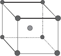
This model does not require a full 3k design, a 2k will do. However, to be safe, it’s best in cases like this to add CPs, replicated at least four times to provide sufficient information on possible curvature in the system. Figure 3.5 shows a picture of this design for three factors (k = 3).
The 2k design (cubical portion) produces eight unique combinations, enough to fit the 2FI model, which contains only seven coefficients. The savings of doing only the 23 versus the full 33 is obviously substantial. However, you get what you pay for: the chosen design will not do much better than OFAT at revealing the sharp curvature shown in the rising ridge in Figure 3.1. That’s where CPs come into play. As we will explain further, although they provide no information for estimating any of the 2FI coefficients, CPs support a test for curvature in the form of pure quadratic terms (A2, B2, C2).
Table 3.2 shows the result of the experiment by the chemist. Note that yield is measured as grams of product made as a result of the reaction. The data are listed in a standard order used for design templates, but the experiment was actually done by randomizing the runs.
Figure 3.5 Two-level factorial design with CP.
Table 3.2 Two-Level Factorial with CPs on Chemical Reaction
Std Ord. |
A: Time (minutes) |
B: Temp. (degree Celcius) |
C: Rate (mL/minutes) |
Yield (grams) |
1 |
80 (−) |
140 (−) |
4 (−) |
76.6 |
2 |
100 (+) |
140 (−) |
4 (−) |
82.5 |
3 |
80 (−) |
150 (+) |
4 (−) |
86.0 |
4 |
100 (+) |
150 (+) |
4 (−) |
75.9 |
5 |
80 (−) |
140 (−) |
6 (+) |
79.1 |
6 |
100 (+) |
140 (−) |
6 (+) |
82.1 |
7 |
80 (−) |
150 (+) |
6 (+) |
88.2 |
8 |
100 (+) |
150 (+) |
6 (+) |
79.0 |
9 |
90 (0) |
145 (0) |
5 (0) |
87.1 |
10 |
90 (0) |
145 (0) |
5 (0) |
85.7 |
11 |
90 (0) |
145 (0) |
5 (0) |
87.8 |
12 |
90 (0) |
145 (0) |
5 (0) |
84.2 |
OBTAINING A TRULY “PURE” ERROR
When viewing the layout of factors in Table 3.2, it’s tempting to actually execute the experiment in the order (standard) shown, especially when it comes to the CPs (listed in rows 9–12). This would be a big mistake, particularly in a continuous (as opposed to batch) reaction, because the variation would be far less this way than if the four runs were done at random intervals throughout the experiment. A proper replication would require that the same steps be taken as for any other run; that is, starting by charging the reactor, then bringing it up to temperature, etc. In our consultancy at Stat-Ease, we’ve come across innumerable examples where so-called “pure error” came out suspiciously low. After questioning our clients on this, we’ve found many causes for incorrect estimates of error (listed in order of grievousness):
 Running replicates one after the other
Rerunning replicates that don’t come out as expected (common when factors are set up according to standard operating procedures)
Taking multiple samples from a given run and terming them “replicates”
Simply retesting a given sample a number of times
Recording the same number over and over
You may scoff at this last misbehavior (known in the chemical industry as “dry-labbing”) but this happened to a Stat-Ease client—a chemist who laid out a well-constructed RSM design to be run in random order by a technician. The ANOVA revealed a pure error of zero. It was overlooked until we pointed out a statistic called “lack of fit” (discussed somewhat in Chapter 1 and in more detail in this chapter), which put the estimate of pure error in the divisor, thus causing the result to be infinite. Upon inspection of the data, we realized that the technician wrote down the same result to many decimal places, so obviously it was thought to be a waste of time rerunning the reaction.
Notice that in Table 3.2, we’ve put the coded levels of each factor in parentheses. The classical (we prefer to call it “standard”) approach to two-level design converts factors to –1 and +1 for low versus high levels, respectively. This facilitates model fitting and coefficient interpretation.
Predictive equations are generally done in coded form so they can be readily interpreted. In this case, the standard method for analysis of 2k designs (see DOE Simplified, Chapter 3) produced the coded equation shown below
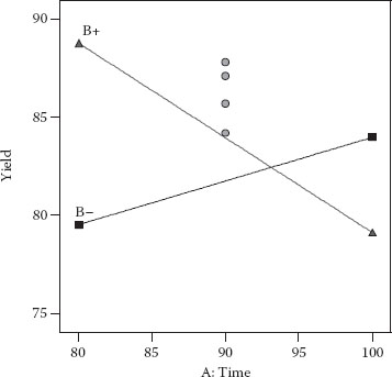
The value for the intercept (β0 = 82.85) represents the average of all actual responses. In coded format, units of measure for the predictors (A, B, and C in this case) become superfluous. Therefore, the model coefficients (β) can be directly compared as a measure of their relative impact. For example, in the equation for yield, note the relatively large interaction between factors A and B and the fact that it’s negative. This indicates an appreciable antagonism between time and temperature. In other words, when both these factors are at the same level, the response drops off. (They don’t get along well together!) The interaction plot for AB is displayed in Figure 3.6.
Figure 3.6 Interaction plot for effect of AB on reaction yield.
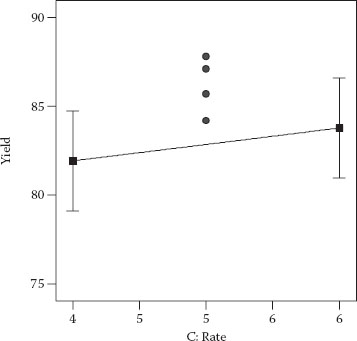
The points in the middle represent results from the four CPs, the values of which can be seen in the last four rows of Table 3.2: 87.1, 85.7, 87.8, and 84.2. The CPs remain at the same levels on the main effect plot (Figure 3.7) for factor C. We included this factor in the model only for illustrative purposes. It was not significant (p > 0.1).
Figure 3.7 Main effect plot for factor C.
ASIDE ON BARS MADE FROM LEAST SIGNIFICANT DIFFERENCE
The effects plot in Figure 3.7 displays a form of confidence interval (CI) called a “least significant difference” (LSD) bar. These particular LSD bars are set to provide 95% confidence in differences. In other words, when the bars do not overlap, you can conclude that the differences in means (end points of graphed lines) are significant. The line showing the C’s effect (Figure 3.7) exhibit overlapping LSD bars from left to right, so the conclusion must be that this difference is not significant. For details on the calculations for the LSD, see DOE Simplified, Chapter 2.
Clearly, from Figures 3.6 and 3.7, these CPs are not fitted very well. They appear to be too high. According to the standard coding scheme (−/+), the CP falls at zero for all factors ([A,B,C] = [0,0,0]). When you plug these coordinates into the coded equation, the result equals the intercept: 82.5. This predicted response for the CP falls below all of the actual values. Something clearly is not right with the factorial model for the reaction yield. It fails to adequately fit what obviously is a curve in the response.
At this stage, we can take advantage of having properly replicated (we hope: see the note titled “More on Degrees of Freedom…”) one or more design points, in this case the ones at the overall centroid of the cubical region of experimentation. (Sorry, but to keep you on your toes, we got a bit geometric there!) The four CP responses produce three measures, statistically termed “degrees of freedom” (df), of variation known as “pure error.” You may infer from this terminology the existence of “impure” error, which is not far off—another estimate of variation comes from the residual left over from the model fitting.
MORE ON DF AND CHOICE OF POINTS TO REPLICATE
In the reactor case, it may appear arbitrary to replicate only the CPs. The same df (3) would’ve been generated by replicating three unique runs, chosen at random. From two responses at a given setup, you get one measure, or degree of freedom, to estimate error. In other words, as a general rule: df = n − 1, where n is the subgroup (or sample) size. Replicating CPs, versus any others, at this stage made most sense because it filled the gap in the middle of the factorial space and enabled a test for curvature (described in the section titled “A Test for Curvature…”). It pays to put the power of replication at this location, around which the factors are varied high and low. By replicating the same point a number of times at random, you also create a variability “barometer” (remember those instruments for pressure with the big easy-to-read dials?). Without doing any fancy statistics, you can simply keep an eye on the results of the same setup repeated over and over, similar to the “control” built in as a safeguard against spurious outcomes in classical experimentation.
A Test for Curvature Tailored to 2k Designs with CPs
We now apply a specific test for curvature that’s geared for 2k designs with CPs. Table 3.3 shows the results of this test, which produces a highly significant p-value of 0.0010.
Let’s delve into the details on how to test for curvature. If no curvature exists, the CPs (inner) on average will differ only insignificantly from the average of the factorial points (outer). Therefore, to assess curvature, the appropriate F-test is
Table 3.3 ANOVA Showing Curvature Test
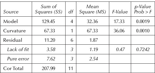
The denominator expresses the variance associated with the squared difference in means as a function of the number (N) of each point type. In the case of the chemical reaction:
The value of 1.87 comes from the mean square residual in the ANOVA (see Table 3.3) above. It’s based on 6 df. The critical value of F for the 1 df of variance in the numerator and 6 df in the denominator is approximately 6, so the value of 36.06 represents highly significant curvature (p = 0.0010). After removing this large source of variance (67.33 SSCurvature) by essentially appending a term for curvature to the model, the LOF becomes insignificant (p > 0.7). The conclusion from all this is that the factorial model fits the outer points (insignificant LOF), but obviously not the inner CPs (significant curvature).
Further Discussion on Testing for Lack of Fit (LOF)
Statistical software that does not explicitly recognize CP curvature in 2k designs produces different results on the ANOVA. Table 3.4 displays the results, which look quite different than before in Table 3.3.
Note the big increase in SS for residuals, specifically those labeled as “Lack of fit.” All of the variation previously removed to account for curvature at the CP pours into this “bucket.” As a result, the model F-value falls precipitously, causing the associated p-value to increase somewhat above acceptable levels for significance. Furthermore, since pure error remains unchanged from the prior ANOVA (Table 3.3), the large variance now exhibited for LOF translates to a much more significant p-value of 0.0712. Recall that a similar situation occurred when trying to fit a linear model to the drive-time data: the p-value for LOF fell below 0.1. This is not good.
Table 3.4 ANOVA with Curvature Added to Error
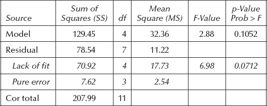
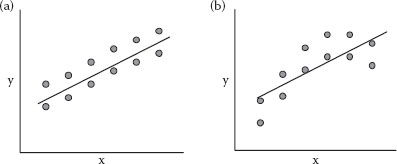
Figure 3.8 (a) LOF not significant. (b) LOF significant.
Figure 3.8a and b illustrates LOF for a simple experiment involving six levels of one factor (x), each of which is replicated for a total of 12 runs.
In Figure 3.8a, an “eye-fit” tells you that all is good. What you see is that the variations of points from the fitted line are about what you’d expect based on variations of the replicate points from their mean (the pure error). This is precisely what’s tested for LOF in ANOVA. However, in Figure 3.8b, it’s immediately obvious that the line does not fit the points adequately. In this case, the deviations from the fitted line significantly exceed what should be expected from the pure error of replication. Although it’s not the only solution, often a better fit can be accomplished by adding more, typically higher order, terms to your model. For example, by adding the x2 term, thus increasing the model order to quadratic, the LOF would be alleviated in Figure 3.8b, because then you’d capture the curvature. Similarly, in the drive-time example, higher-order terms ultimately got the job done for producing an adequate representation of the true surface.
The Fork in the Road Has Been Reached!
Now we see that a price must be paid for not completing the full 33 (=27 run) design for the chemical reaction experiment. ANOVA (in Table 3.3) for the two-level design shows highly significant curvature. However, because all factors, rather than each individually, are run at their mid-levels via CPs, we cannot say whether the observed curvature occurs in the A, B, or C factors or some combination thereof. For example, perhaps the main effect of C is very weak because the response goes up in the middle before dropping off. In this scenario, adding a term for C2 would capture the evident curvature. However, it would be equally plausible to speculate that the curvature occurs as a function of both A and B in a way that would describe a rising ridge. In this case, the squared terms for these two factors would be added to the predictive model.
Statisticians call this confounding of curvature an “alias” relationship—described mathematically as
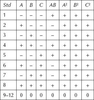
Even a statistician cannot separate the squared terms. Table 3.5 illustrates why. It shows the 23 design with CPs with factor levels coded according to the standard scheme: minus (–) for low, plus (+) for high, and zero (0) for center. The pattern for the three control factors (A, B, and C) is laid out in standard order. Their effects are calculated using the response data aligned with the pluses versus the minuses.
Higher-order factorial terms such as AB can be estimated by first multiplying the parent terms, in these cases A and B, to create a new column and then calculating the coefficients. However, applying this same procedure to the squared terms does little good, because they all come out the same.
Table 3.5 Aliasing of Squared Terms in Two-Level Factorial with CPs
LADIES TASTING TEA VERSUS GIRLS GULPING COLA
The development of modern-day DOE is generally credited to Sir Ronald Fisher (1890–1962), a geneticist who developed statistical tools, most notably ANOVA, for testing crops. He developed the concept of randomization as a protection against lurking variables prevalent in agricultural environments and elsewhere. Fisher discusses randomization and replication at length in his classic article, “Mathematics of a Lady Tasting Tea” (reprinted most recently in Newman’s The World of Mathematics, Vol. 3, Dover Press, 2000). Fisher’s premise is that a lady claims to have the ability to tell which went into her cup first—the tea or the milk. He devised a test whereupon the lady is presented eight cups in random order, four of which are made one way (tea first) and four the other (milk first). Fisher calculates the odds of correct identification as one right way out of 70 possible selections, which falls below the standard 5% probability value generally accepted for statistical significance. However, being a gentleman, Fisher does not reveal whether the lady makes good on her boast of being an expert on tea tasting.
The experiment on tea is fairly simple, but it illustrates important concepts of DOE, particularly the care that must be taken not to confound factors such as what you taste versus run order. For example, as an elementary science project on taste perception, Mark’s youngest daughter asked him and several other family members to compare two major brands of cola-flavored carbonated beverages. She knew from discussion in school that consumers often harbor biases, so the taste test made use of unmarked cups for a blind comparison. Unfortunately, this neophyte experimenter put one brand of cola in white Styrofoam® cups and the other in blue plastic glasses in order to keep them straight. Obviously, this created an aliasing of container type with beverage brand. Nothing could be done statistically to eliminate the resulting confusion about consumer preferences. Don’t do this at home (or at work)!
To consult a statistician after an experiment is finished is often merely to ask him to conduct a postmortem examination. He can perhaps say what the experiment died of.
R.A. Fisher
Presidential Address to the First Indian
Statistical Congress, 1938
It will take more experimentation to pin down the source of curvature in the response from the chemical reaction. In the next chapter we will present part two of this case study, which involves augmenting the existing design with a second block of runs. By adding a number of unique factor combinations, the predictive model can be dealiased in terms of A2, B2, and C2—the potential sources for pure curvature.
PRACTICE PROBLEMS
3.1 From the website from which you downloaded the program associated with this book, open the tutorial titled “*Two-level Factorial*”.pdf (* signifies other characters in the file names). You might find several files with this title embedded—pick the one that comes first in sequential order (“Part 1”) and follow the instructions. This tutorial demonstrates the use of software for two-level factorial designs. The data you will analyze come from Montgomery (2012). He reported on a waferboard manufacturer who needed to reduce concentration of formaldehyde used as processing aid for a filtration operation. Table 3.6 shows the design sorted by standard order.
You will be well served by mastering two-level factorials such as this before taking on RSM. Obviously, if you will be using Design-Expert® software, the tutorial will be extremely helpful. However, even if you end up using different program, you will still benefit by poring over the details provided on the design and analysis of experiments.
3.2 In Chapter 8 of DOE Simplified, we describe an experiment on confetti made by cutting strips of paper to the following dimensions:
a. Width, inches: 1–3
b. Height, inches: 3–5
The two-level design with CPs is shown below with the resulting flight times (Table 3.7).
Each strand was dropped 10 times and then the results were averaged. These are considered to be duplicates rather than true replicates because some operations are not repeated, such as the cutting of the paper. On the other hand, we show four separate runs of CPs (standard orders 5–8), which were replicated by repeating all process steps, that is, recutting the confetti to specified dimensions four times, not simply redropping the same piece four times. Thus, the variation within CPs provides an accurate estimate of the “pure error” of the confetti production process. Set up and analyze this data. Do you see significant curvature?
Table 3.6 Data from Montgomery Case Study
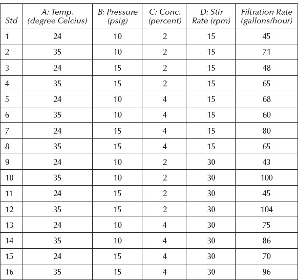
Table 3.7 Flight Times for Confetti Made to Varying Dimensions
Std |
A: Width (inches) |
B: Length (inches) |
Time (seconds) |
1 |
1 |
3 |
2.5 |
2 |
3 |
3 |
1.9 |
3 |
1 |
5 |
2.8 |
4 |
3 |
5 |
2.0 |
5 |
2 |
4 |
2.8 |
6 |
2 |
4 |
2.7 |
7 |
2 |
4 |
2.6 |
8 |
2 |
4 |
2.7 |
FLYING OFF TO WILD BLUE YONDER VIA “METHOD OF STEEPEST ASCENT”
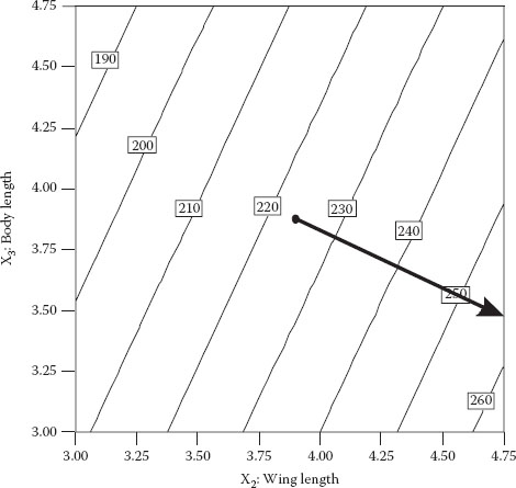
Box and Liu (1998) report on a fun and informative series of experiments involving optimization of paper helicopters. They apply standard strategies for DOE with a bit of derring-do en route—the method of steepest ascent (Box and Wilson, 1951). This is an aggressive approach that involves taking some risky moves into the unknown, but hopefully in the right direction. It is normally done only at the early phases of process or product improvement—when you are still at the planar stage, far from the peak of performance. If a linear model suffices for predictive purposes, the procedure is made easy with the aid of response surface plots: make moves perpendicular to the contours in the uphill or downhill direction, whichever you seek for optimum outcome. Figure 3.9 illustrates this for an experiment on paper helicopters reported by Box and Liu.
In their example, an initial two-level screening design produces the following linear model of mean flight times (in centiseconds):
Only the three factors shown came out significant, out of eight originally tested.
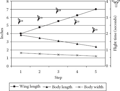
The path of steepest ascent can now be calculated by starting at the center of the original design and changing factors in proportion to the coefficients of the coded fitted equation. In the case of the helicopter, the path was moved along a vector that went up 28 units in x2 (wing length), down 13 units in x3 (body length), and down 8 units in x4 (body width). Box and Liu took off in this direction with redesign of their helicopters and found that flight times peaked at the third step out of five (see Figure 3.10).
They stopped at this point and did a full, two-level factorial on the key factors. Eventually, after a series of iterative experiments, culminating with RSM, a helicopter is designed that flies consistently for over 4 seconds.
The method of steepest ascent is just one element in what Box and Liu call “…a process of iterative learning [that] can …start from different places and follow different routes and yet have a good chance of converging on some satisfactory solution…”
Figure 3.9 Direction of steepest ascent.
Figure 3.10 Step-by step helicopter dimensions (left axis) versus flight times (right axis).