Chapter 8

Everything You Should Know about CCDs (but Dare Not Ask!)

Theory guides, experiment decides.

I.M. Kolthoff

University of Minnesota professor known as the father of analytical chemistry

From the very beginning (Box and Wilson, 1951), statisticians have debated criteria for the ideal structure of the CCD, in particular, the number of CPs per block and how far out the axial levels (star points) should go. In this chapter, we will discuss what’s good in theory versus more practical considerations for real-life experimentation.

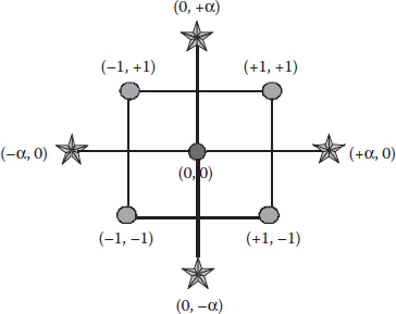
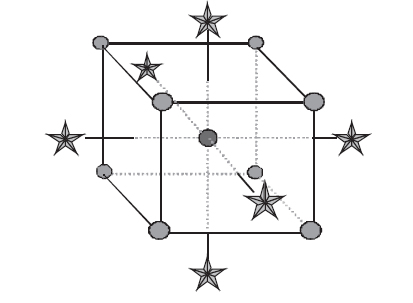
Let’s start by tackling the toughest issue for experimenters wanting to do RSM via CCDs—where to place their star points. For over half a century, the dogma has been that stars must go outside of the factorial box as shown in Figure 8.1.

Going to these extremes offers advantages, the most obvious of which is the greater leverage for estimating the main effects and curvature. The main disadvantage of venturing outside the box is equally obvious—the stars may break the envelope of what’s safe or even physically possible. For example, what if you include a factor such as a dimension of a physical part and the lower star point comes out negative? Or, worse yet, the equipment may fail catastrophically when certain operating limits are exceeded at the upper star points. There’s a more subtle disadvantage to the standard construction for the CCD; experimenters often find it inconvenient to adjust their process to the five levels required of each factor:

Figure 8.1  Standard CCD with stars outside of the box.

  A low axial (a star at the lowest level)

  A low factorial

  A CP

  A high factorial

  A high axial (a star at the highest level)

Therefore, as we mentioned briefly in Chapter 4, the experimenter may opt to do an FCD (see Figure 4.2).

Now that you know you don’t have to go to the extremes shown in Figure 8.1, it may be easier to remain open-minded about the possibilities. Let’s get into the statistical details on why Box and Wilson were so keen for you to do this and determine exactly where they wanted to put the stars (and why). When constructed properly, the CCD provides a solid foundation for generating a response surface map by providing the necessary runs to fit a quadratic polynomial. Figure 8.2 lays out the geometry for a generic CCD on two factors.

A CCD always contains twice as many star points as there are factors in the design. The axial distances to the star points are designated by the Greek symbol alpha (α). They are measured in terms of coded units, where plus-or-minus 1 represents the factorial ranges. Typically, the alpha value varies from 1 (the face-centered option) to the square root of the number of factors (√k), which produces a spherical geometry. However, even higher values may be chosen. For example, Box and Draper (1987, pp. 305–311) show a CCD for three factors with the star points placed at plus-or-minus 2 (>√3 = 1.73). Myers et al. (2016, p. 395) also present a three-factor case, but they put the stars to 1.682 units from the CP. Oddly enough, in the CCD example detailed in Chapter 4, the coded alpha value of 1.682 was used to generate the star points for the three factors (see Table 4.1 for the actual levels). Why use such an odd value: 1.682? It turns out that at this particular placement of the star points, a CCD with three factors exhibits a feature much coveted by statisticians—rotatability.

Figure 8.2  Coded levels for CCD.

THE FATHER OF QUADRATIC EQUATIONS

Diophantus was an Alexandrian (Egypt) whom many consider to be the father of algebra. He is best known for his text Arithmetica, which presented the solution for quadratic equations—the primary model for RSM. Historians know very little about his life or even when he lived other than it was in the early centuries A.D. Even his epitaph is a puzzle (Newman, 1956), but if you are adept with fractions, it reveals Diophantus’s age at death:

…God vouchsafed that he should be a boy for the sixth part of his life; when a twelfth was added, his cheeks acquired a beard; He kindled for him the light of marriage after a seventh, and in the fifth year after his marriage He granted him a son. Alas, late-begotten and miserable child, when he [Diophantus’s son] had reached the measure of half his father’s life, the chill grave took him. After consoling his grief by this science of numbers for four years, he [Diophantus] reached the end of his life.

Can you figure out how long Diophantus lived? (Hint: determine the common denominator for the three fractions of his life before getting married.)

Rotatable Central Composite Designs (CCDs)

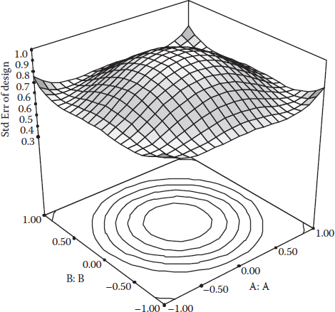
Rotatability—what’s in it for you? Well, first of all, recall from Chapter 4 that the standard error plot (Figure 4.9a and b) for the design we held up as a sterling RSM exhibited perfectly circular contours, which indicates that equally precise predictions will be obtained at any location equally distant from the CP of the experimental space. Any other pattern would indicate that the design favors moving from your bull’s eye at the middle in one direction versus another, thus indicating a bias on the part of the experimenter. As you’ve learned by now, bias is a four-letter word in statistical jargon, one that must be avoided if at all possible.

Consider an example of a nonrotatable design—a full three-level factorial. The standard error plot for a 3² design (nine runs, only one at a CP) can be seen in Figure 8.3.

Figure 8.3  Standard error plot for a three-level design (nonrotatable).

First of all, notice that the projected contours are not circular, thus indicating nonrotatability. However, as a more practical matter, you see that there are four well-predicted pockets at regions that probably hold no more interest for the experimenter than any other combination of factors.

ROUND AND ROUND ON ROTATABILITY: SOME DIZZYING DETAILS

Box and Hunter (1957) were the first DOE experts to tout rotatability as a desirable feature for RSM. To generate this property in a CCD, the value of alpha must conform to the following function:

$\text{α}={[2^{(\text{k}-\text{p})}]}^{1/4}$

Recall that 2^k−p specifies a two-level design on k factors, where minus p represents the fraction. In other words, for a CCD to be rotatable, the coded axial distance of its star points must equate to the fourth root of the number of experimental runs in the two-level factorial portion. Designs conforming to this specification will generally place the factorial points and star points on different spheres. For example, a three-factor CCD puts stars at plus-or-minus 1.68 coded units (=[2³]^1/4 = 8^1/4) versus a radius for cube points of 1.73. Thus, this design, like most rotatable CCDs, is not equiradial.

So long as we’re going around in circles in this sidebar, it’s worth noting, while on the topic of equiradial geometry that this does describe a class of rotatable RSM designs for two factors, the most popular of which is the hexagon, featuring six evenly spaced points in a circle, plus a number of CPs. The minimum-run equiradial design for fitting a quadratic polynomial is the pentagon, but this should be avoided due to having points with a leverage of 1. (Perhaps, such a dangerous design should be left to experimenters working on behalf of the U.S. Defense Department, who make their home in the famous Washington, DC building of the same geometry.) A special case of an equiradial design is the octagon, which doubles as the two-factor rotatable CCD; so, it gets used quite often by practitioners of RSM.

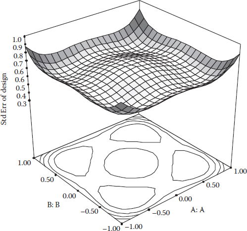
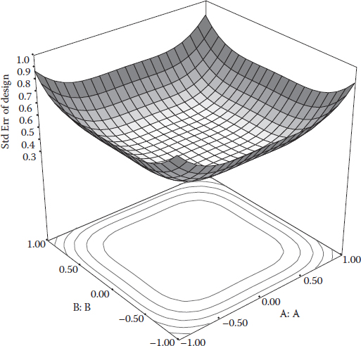
A much better alternative is the two-factor CCD pictured in Figure 8.4 with a rotatable alpha value of 1.414 and four replicates of the CP (five in all). Notice in Figure 8.4 how the standard error for prediction, plotted to the same scale as before, now exhibits symmetry.

Figure 8.4  Standard error plot for a two-factor rotatable CCD.

Also, by bulking up on the CPs, the error for response prediction is minimized in the bulls-eye region and it increases only gradually until you get very near the factorial boundaries (±1 coded unit from the center). We advise that you be wary when wandering outside of this box because of the rapid increase in standard error, and dangers of extrapolating into space that’s only been “scouted” by the venturesome stars. However, as suggested in Chapter 4’s not “Going Outside the Box,” after running a rotatable CCD, you will do well by moving beyond the factorial limits to the standard error limit set by these points.

Going Cuboidal When Your Region of Operability and Interest Coincide

Here is a communication (Anderson, 2001) with an actual experimenter that raises some practical questions about where to place star points in a CCD:

I am having a tough time trying to decide between two CCDs, one with alpha of 1.682 [rotatable] and the other with alpha of 1 [face-centered]. I have three factors, each of which can vary from 0 to 100. Negative values are inadmissible. Therefore, I generated the first [rotatable] design by setting factor ranges in terms of alpha.

Figure 8.5  Rotatable CCD fit into a cubical region of operability.

In this case, the experimenter’s region of operability (0–100) and the region of interest coincide. Imagine trying to force fit the rotatable three-factor CCD (coded alpha = 1.682) into a cubical cage with each side of 100 actual units in length. The factorial cube is now pushed well within the middle of the region of interest (see Figure 8.5).

Clearly, only a minor portion of the region of operation/interest will be explored by the RSM design, specifically (1/1.682)³ or 0.21. In other words, nearly 80% of the region of interest is left relatively unexplored.

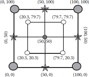
Now, we see that the experimenter’s idea of doing an FCD makes much more sense. By looking at a two-factor projection of the 3D region, Figure 8.6 provides a comparative view of the FCD versus CCD inscribed within the operating limits of 0–100.

Figure 8.6  FCD versus CCD.

The smaller square made up of open circles is the factorial region abandoned from the rotatable CCD in favor of the larger, solid-pointed factorial part of the FCD that now fills out the operating envelope. You may be wondering about the odd settings of 20.3 and 79.7 for the CCD. A bit of arithmetic solves this mystery:

1.  Start by working out the conversion from actual to coded units. To be rotatable, the stars are placed on 1.682 coded units that are out from the (50, 50) CP. They span 0–100 on the actual scale. Thus, 1.682 coded units convert into 50 (100–50 or 50–0) actual units.

2.  Convert the plus-or-minus one factorial levels into actual ranges: 50/1.682 = 29.7.

3.  Add and subtract this value from the actual coordinates at the CP to get the values of 79.7 (=50 + 29.7) and 20.3 (=50 – 29.7).

This bother is alleviated by the use of software that will set up CCDs, but that still leaves the inconvenient settings to be run on the process—all the more reason to abandon this design in favor of the FCD.

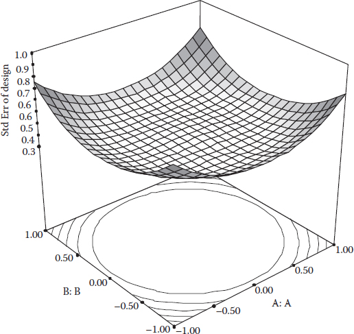
Of course, everyone knows that you cannot put a square peg in a round hole, or in this case, expect a cube to fill a sphere. By changing alpha to 1, you pull the axial points into the face of the cube, which creates a design that’s no longer rotatable (spherical standard error contours) but rather cuboidal, as can be seen in Figure 8.7, which depicts the standard error (plotted to the same scale as the previous plots) for the FCD discussed above (pictured in Figure 8.6).

In conclusion, for five or fewer factors, we advise you to make use of an FCD, rather than a rotatable CCD, when you want to explore the entire region of process operability. As we will detail later in a sidebar called “Dampening Inflation of Variance,” at larger numbers of factors (>5), FCDs exhibit an excessive collinearity among the squared terms, which can be quantified via their VIFs. You may be tempted to try a BBD for situations like this. However, be aware that this is not a cuboidal design because, as we illustrated in Figure 5.1, it will not put points at the corners of your space. (Sorry, we really would like to keep RSM simple, but at least, we waited until this “everything you should know” stage to delve into all the pros and cons of various ways of constructing CCDs. We must assume that if you’re still reading this book, you remain undaunted and dare ask about such things.)

Figure 8.7  Cuboidal standard error for FCD.

CUBOIDAL SPACES FOR THE OFFICE (A TIME-OUT FROM STAT STUFF)

If you work for a large corporation that keeps you cooped up in a cubicle, take a break from all this humdrum and rent or stream the movie Office Space, written and directed by Mike Judge, Twentieth Century Fox (1999). To avoid the closed-in feeling of myriad cuboidal spaces, one high-tech Californian client of the authors eliminated all walls and outlawed all opaque furnishings. It featured mesh-backed chairs and desks made out of wire. Perhaps, cubes aren’t that bad after all!

We don’t have a lot of time on this earth! We weren’t meant to spend it this way. Human beings were not meant to sit in little cubicles staring at computer screens all day… filling out useless forms… and listening to eight different bosses drone on about mission statements.

Spoken by one of the oppressed workers in Office Space

Practical Placement of Stars: Outside the Box but Still in the Galaxy

Let’s go back to the drawing board on CCDs by assuming that operating limits do not impose constraints on the region of interest. Furthermore, we ought to consider expanding these RSMs to more than just two or three factors. Robotic equipment, often at very small scales, now makes it feasible to simultaneously vary many factors, perhaps dozens. In many cases, there is no physical process: its essence is captured in a complex, black-box computer simulation that requires experiments for model development. Surely, Box and Wilson never anticipated this technology when they invented the CCD in 1951. To get a handle on the problem, observe in Table 8.1 what happens to the rotatable alpha level as the number of factors (k) escalates.

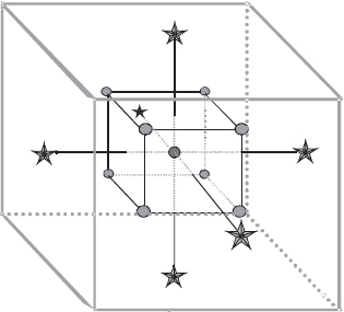
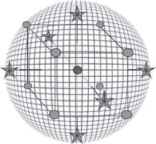
To keep the number of runs from exploding, we’ve applied a fraction (p) to the core factorials. For example, for 10 factors, the fractional factorial is 2⁻³ or 1/8th of the 512 runs needed to do all the full number of two-level combinations. As p increases, the alpha level for rotatability decreases (see the earlier note titled “Round and Round on Rotatability…” for the formula), but even so, it remains so far out that one must question its practicality. Myers et al. (2016, p. 406) propose setting alpha at the square root of the number of factors (√k) to create a spherical design such as that shown in Figure 8.8.

However, as you can see in Table 8.1, this spherical specification for the star points achieves KISS (keeping it simple, statistically), but does not make them any more practical.

We propose a much more radical paring of the alpha level for star points: fourth root of the number of factors (k^1/4). The results of this calculation can be seen in the last column of Table 8.1. As discussed in the sidebar “Dampening Inflation of Variance,” this design specification offers a good tradeoff of practicality versus statistical properties.

Table 8.1  Impact of Increasing Factors on Star-Point Placement

k	p	Rot. α	α = k1/2	α = k1/4
2	0	1.414	1.414	1.189
5	1	2.000	2.236	1.495
10	3	3.364	3.162	1.778
20	11	4.757	4.472	2.115

Figure 8.8  Spherical CCD.

DAMPENING INFLATION OF VARIANCE

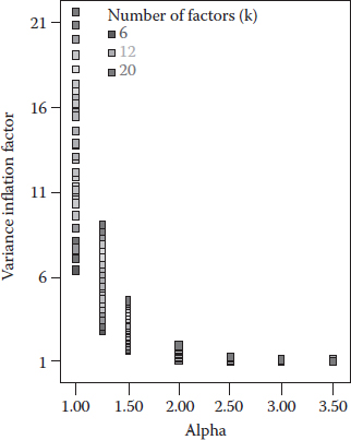
As stars in a CCD get pulled into the face of the factorial hypercube, the VIFs for the quadratic terms (x_i²) increase, thus making it harder to estimate their model coefficients. Fortunately, the VIFs are dampened considerably by only a small increase in alpha levels above the face-centered value of 1. This is illustrated in Figure 8.9, which shows how VIF varies as a function of alpha and k—the number of factors from 6 to 20, in some cases with more than one result shown due to options on how far to fractionate the core factorial. As a rough rule of thumb, the VIF at alpha 1.00 equals the number of factors. Although it’s not that relevant to our conclusions, this should help you to interpret the shades of gray keyed to k.

Figure 8.9  VIFs as a function of alpha and k.

Here’s another rule of thumb: VIFs above 10 indicate an unacceptably high multicollinearity (Montgomery, Peck, and Vining, p. 119). On this basis, it can be inferred from the graph that an FCD (α = 1.00) will not be a good choice unless dictated by operating constraints. Our initial thought for KISS was to fix alpha at a level of 1.50 where VIFs fall well below the level of 10. But as a refinement to counteract the higher VIFs for designs with many factors (k ≥ 6), we suggest setting alpha on the basis of the fourth root of k, if practical, but not less than 1.5.

For more details, see Whitcomb and Anderson (2003), posted at www.statease.com/publications/case-studies/practical-versus-statistical-aspects-of-alternating-central-composite-designs.html.

CPs in Central Composite Designs

Our clients often ask if it would be alright to cut down or possibly even eliminate the replication of CPs called for by textbooks and associated software for CCDs. In short, the answer is “No!”

Recall from the previous chapter that a good RSM design should provide for testing of LOF. Otherwise, you cannot tell how well your model fits the actual response data. This statistic requires a measure of pure error, which comes only from true replication. To achieve any sort of reasonable power for the LOF test, three df of pure error are mandatory. If only CPs are replicated, then, you must do at least four of them to get over this threshold.

GETTING OVER THE HURDLE OF CRITICAL F-VALUES

With fewer than four df, the LOF test achieves very little power, in part due to the rapid escalation of critical F-values with such meager samples of data. For example, consider doing a three-factor CCD. For uniform precision, we suggest that this design includes six CPs, but you may be tempted to do fewer. Think again after seeing these critical F-values at the 5% risk level as a function of the number of “CPs”:

CPs	df	F(5,df) for LOF
1	0	Not possible
2	1	230.2
3	2	19.30
4	3	9.01
5	4	6.26
6	5	5.05

To construct this table, we assumed a full quadratic model that leaves five df for a residual to test against many df of pure error for the F-test on LOF. Notice how it stabilizes at four df and beyond.

Furthermore, as we discuss in Appendix 8A at the end of this chapter, if the CCD is broken up into blocks and you desire them to be orthogonal, the number of CPs not only increases, but they must also be split into different design segments in a specific manner.

Despite all these admonitions, nonstatistical industrial experimenters generally persist in viewing the replication of CPs to be a waste of valuable time and resources. Let’s look at this controversy from another angle—uniformity of precision for response predictions. As you’ve seen in Figures 8.4 and 8.7, a well-constructed CCD or FCD provides a relatively flat and low standard error throughout the middle of the factorial region. On the other hand, as you can see in Figure 8.10, cutting back on the number of CPs degrades this uniformly precise pattern of standard error (plotted to the same scale as before). It shows what happens if you cut back to only one CP from the five in the original two-factor rotatable CCD illustrated in Figure 8.4.

Flip back and forth between Figures 8.4 and 8.10. Enough said?

Final Comments: How We Recommend That You Construct CCDs

So now, you know a lot more about the construction of CCDs than you ever wanted to learn. Unless you are a statistician (who laps up this kind of stuff), it’s likely that at this stage you suffer from TMI. Therefore, we decided that it would be merciful to try summarizing our recommendations on CCDs.

Figure 8.10  Standard error plot for a two-factor rotatable CCD with only one CP.

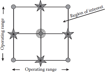
First of all, you must consider how your region of interest relates to the operating boundaries for the experimental factors. For example, consider the situation pictured in Figure 8.11.

It depicts an FCD (equivalent in this case to a full three-level design) for two factors held within operating limits. The circles around the CP show that it’s replicated a number of times—we recommend five for a good test on LOF. In cases such as this, where the regions of interest and operation coincide, we recommend the FCD.

Figure 8.11  Region of interest versus operability.

On the other hand, when operating limits do not come into play relative to the factor ranges you wish to explore; in other words, you will not be pressing against the process envelope, the more traditional form of CCD, with star points outside the box, which will provide much improved predictive properties. However, to keep the range of these wayward stars within a realistic striking distance, we recommend setting them at the fourth root of the number of factors (α = k^1/4). At this setting of alpha, the design will remain nearly rotatable but it will not waste nearly as much space as at the exactly rotatable level. For example, recall that the standard three-factor CCD (α = 1.6823) restricted the ideal volume for prediction (inside the factorial box) to about 1/5th ([1/1.6823]³ = 0.21) of the overall region spanned by the star points. At the lesser value of alpha that we recommend (k = 3^1/4 = 1.316), this region of interest expands to nearly one-half ([1/1.316]³ = 0.44) of the overall experimental volume.

The number of CPs in CCDs should never be less than five in our opinion. The more, the better, particularly as the number of factors increases. Ideally, sufficient replication of CPs can be done to achieve a relatively uniform precision inside the factorial ranges. However, although more research is needed in this area, it may take some multiple of the number of factors to accomplish this objective. For now, to KISS, we advise increasing the replication of CPs to 2 times the number of factors (2k), but capping the number at 10. So, for example, eight CPs in a four-factor CCD might be a practical number.

YET ANOTHER OPTION: ORTHOGONAL QUADRATIC CCDs

We cannot leave well enough alone on all the permutations for setting up CCDs; so, we ask you to consider one more: choosing the alpha level for the star points in such a manner that perfects the VIF for the quadratic terms (x_i²). Achieving VIFs of 1 makes these model coefficients for estimating curvature orthogonal to the main effect and the 2FI term. For example, by setting alpha to 1.414 (√2) on a two-factor CCD, you make it rotatable, but the VIFs for A² and B² are 1.02, which is not quite perfect. If you adhere to the philosophy (paraphrasing George Box) “when doing something really worthwhile you may as well do it right,” and you believe orthogonality is of utmost importance, then, you must set the alpha level at 1.2671 for a two-factor CCD with five CPs. We won’t go into the details,^* but by increasing the CPs on the design to eight, the alpha for orthogonality of the quadratic terms increases to 1.414 and then the design is also rotatable.

*  This criterion for setting alpha was brought up originally by Box and Wilson in the landmark paper on RSM in 1951. If you really want to learn more on the topic, see their paper cited in the references for this book.

PRACTICE PROBLEMS

8.1  University of Minnesota food scientists (Richert et al., 1974) used a CCD to study the effects of five factors on whey protein concentrates, a popular diet supplement for body builders. Also, whey proteins, when properly processed, are beneficial in the development of foams characteristic of frozen desserts, whipped toppings, meringues, and mousses.

WHERE THERE’S A WHEY

Whey is the watery part (called the “serum”) of milk that is separated from the curd in making cheese. Unless you work in the dairy industry (or engage in body building), your only familiarity with this term may be from the nursery rhyme:

Little Miss Muffet, sat on a tuffet,

Eating her curds and whey.

Along came a spider,

Who sat down beside her

And frightened Miss Muffet away.

P.S. A “tuffet” is either a mound of earth or a three-legged stool. (Source: http://sircourtlynice.blogspot.com/2010/09/tuffets-and-how-to-sit-on-them.html.)

The factors, with ranges noted in terms of alpha (star levels), were

A.  Heating temperature: 65–85 degree celsius per 30 minutes

B.  pH level: 4–8

C.  Redox potential: −0.025 to 0.375 volts

D.  Sodium oxalate (Na “Ox”): 0–0.05 molar

E.  Sodium lauryl sulfate (Na LS): 0%–0.2% of solids

There were nine responses, but we will look at only three

1.  Whipping time in minutes (to produce a given amount of foam)

2.  Time at the first drop in minutes (a measure of foam stability)

3.  Undenatured protein in percent

Denature means to render unfit, therefore, the undenatured protein must be maximized. The whipping time should be minimized and the stability maximized.

The experimenters chose a rotatable CCD based on a one-half fraction for the cube portion (2⁵⁻¹). The data are shown in Table 8.2. Be careful when you set up this CCD—all points must fall within the specified ranges. If supported by your software (it is in the one provided with this book), enter the limits in terms of the alpha levels, which are the axial (star) points.

This is a popular design (e.g., it was also used by GE scientists to study plastic processing as presented in Problem 6.2). However, as we discussed in this chapter, rotatable CCDs do a poor job of exploring the x-space, that is, the region defined by the process limits. What would have been a good alternative for these food scientists studying the production of whey protein concentrates?

Develop predictive models for the three responses of interest. With these many factors (five), you may discover that many terms become insignificant in the ANOVA. Therefore, we suggest you to apply model reduction. We did this in Chapter 2 for the Longley data and discussed the pros and cons of it in the sidebar titled “Are You a ‘Tosser’ or a ‘Keeper’?” in Chapter 4. Recall our advice that you be vigilant for cases where a factor and its dependents (e.g., A, AB, AC, and A²) are all insignificant. Is it possible to model any or all of the whey protein responses with only a subset of the tested factors—in other words, one or more factors reduced out of the model? If so, this will simplify the response surfaces and keep things simpler all around.

Also, do not be shy about applying response transformations. By now, you’ve seen this done numerous times throughout the book to produce better predictive models.

Table 8.3 provides criteria for a multiple-response optimization of the process for making whey protein concentrate.

Can you find a sweet spot for the meringue and mousse lovers?

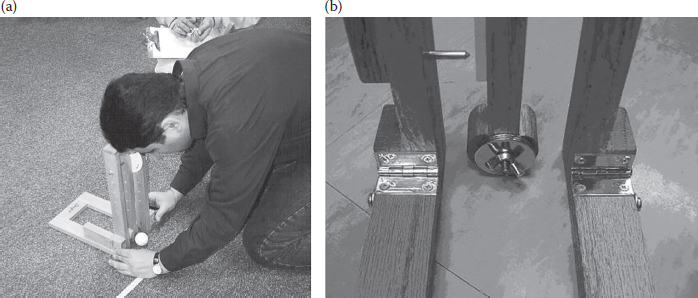
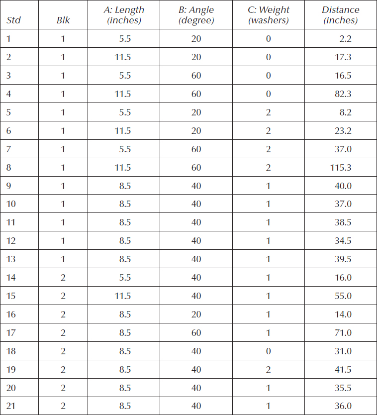
8.2  Leonard Lye, a professor of engineering and applied science at Memorial University of Newfoundland, contributed the following case study. It is based on the DOE Golfer, a machine he invented to teach RSM.
Figure 8.12a shows a student preparing a putt with the DOE Golfer. The weight of the club head can be adjusted by adding washers as shown in the close-up of the golfing machine in Figure 8.12b.

Table 8.2  Data for Whey Protein Study

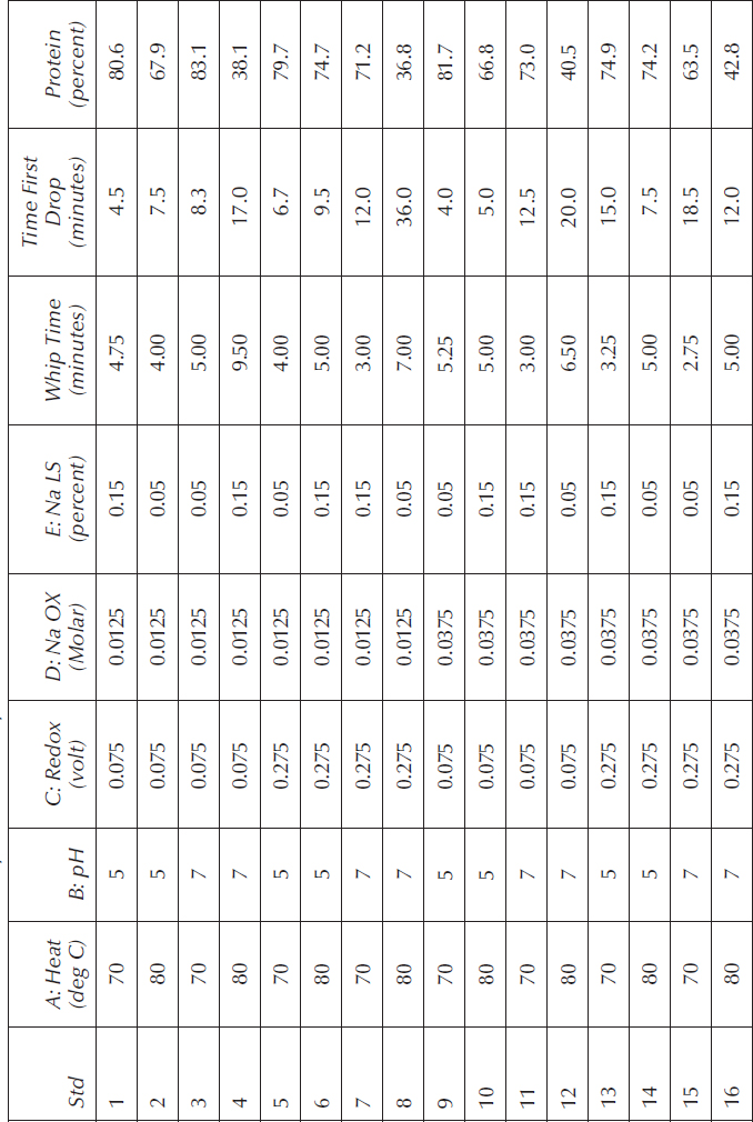
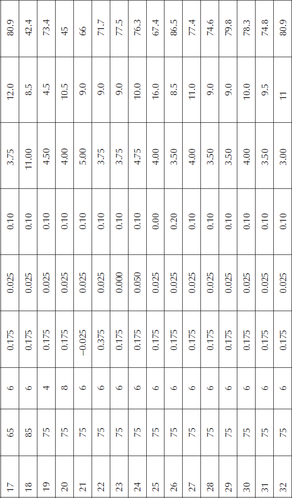
Table 8.3  Multiple-Response Optimization Criteria for Whey Protein Concentrate

Response	Goal	Lower Limit	Upper Limit	Importance
Whip time	Minimize	1	4	++
Time first drop	Maximize	10	20	+++
Protein	Maximize	80	100	++++

Figure 8.12  (a) Student setting up a golf machine. (b) Golf machine club head.

Many factors can be varied in the DOE Golfer, including length of the club, angle of swing, weight of the club, and the type of ball. Table 8.4 shows an experiment conducted on the golfing machine by a group of students who studied three of these four factors. They ended up doing an FCD in two blocks.

Notice that the first block is a full two-level factorial (2³) with five CPs. What did the students see from the analysis of this block alone that led them to augment it with a second block of six face-centered star points (standard-order rows 14 through 19) plus two more CPs (20, 21)? (Hint: do a square root transformation on the response.) On the basis of the predictive model generated from this RSM, what would be a good setup for a six-foot (72-inch) putt with the DOE Golfer, assuming you can give or take 2 inches?

Table 8.4  FCD Done on DOE Golfer

BECOMING AN ACE AT DOING DOE

For bonus marks in his graduate DOE course, Professor Lye organized a golf tournament in the carpeted faculty lounge. Evidently, the grain of this “green” proved to be a decisive factor according to his report on the outcome:

The group that won the tournament clearly had the best design and was the most meticulous. They noticed that direction is important. Going north-to-south is different from going south-to-north, etc. The winners took this into account and that made quite a difference. They even got a hole-in-one for one hole and the maximum number of strokes they needed for any hole was two. It was amazing really.

Other groups needed more than 5 or 6 strokes for one hole. Their first stroke usually got them fairly close to the hole (maybe 2 inches away), but some groups completely forgot about this possibility and failed to develop a proper model for this short distance. Also, if they overshot with the first stroke, the next one had to come from the opposite direction. If the students did not consider direction as a factor, then their prediction was not accurate.

The winning group considered all these possibilities. The moral here is not to assume that the floor is flat or the carpet is uniform in all directions.

(For more details on the DOE Golfer and how you can buy one for educational purposes, see www.statease.com/golftoy.html.)

Appendix 8A: Some Details on Blocking CCDs and Issues of Orthogonality

One of the more practical features built into CCDs by Box and Wilson is their ability to be built up block by block. This can be likened to modular construction of prefab units for customized housing—build only what you really need to cover the required space. For example, the three-factor CCD described in Chapter 4 actually began with a block of 12 factorial runs detailed in Chapter 3. A second block of eight runs was required to make it an RSM design, thus allowing proper modeling of the curvature. As discussed, this three-factor CCD was rotatable. However, it comes up to just the tiniest bit short of achieving orthogonal blocking.

Technically, an RSM is said to be orthogonally blocked if it is divided into segments in such a manner that block effects do not affect the coefficient estimates for the second-order (quadratic) model. This can be quantified in terms of the correlation (r); a value of zero (r = 0) indicates orthogonality. In this case, design evaluation reveals a 0.028 correlation between the block coefficient (included in the predictive model as a correction factor for changes from one time frame to the other) and each of the squared terms (A², B², and C²). For what it’s worth (not much!), by reducing the axial distance of the star points very slightly from the rotatable level of 1.68 to a value of 1.63, this troublesome (only to certain statisticians!) correlation could be eliminated (zeroed out). (Of course, this makes the resulting design imperceptibly nonrotatable.)

In general, for a CCD with k factors done in two blocks (factorial points in one and axial in the other) to be orthogonal, the star points must be set at

$\text{α}=\sqrt{\text{k}\left[\frac{1+({\text{n}}_{\text{s}0}/2\text{k}}{1+({\text{n}}_{\text{f}0}/2^{\text{k}-\text{p}}}\right]}$

where n_s0 and n_f0 are the number of CPs in the axial and factorial blocks, respectively. Since the terms 2k and 2^k−p represent the number of star points and factorial points, respectively, you can see that the orthogonal choice for alpha boils down to a function of the number of factors and the ratio of CPs to other points in each of the two blocks. Solving for the three-factor example we get

$\text{α}=\sqrt{\text{3}\left[\frac{1+(2/2*3)}{1+(4/2^{3-0})}\right]}=\sqrt{\text{3}\left[\frac{1+(2/6)}{1+(4/8)}\right]}=1.632$

In some cases, CCDs can be set up with an alpha value that achieves both rotatability and orthogonality (Ah…sleep at last for the RSM perfectionist!). For example, consider the four-factor design broken up into either two or three blocks as follows:

1.  16 (2⁴) factorial points plus four CPs

2.  8 (2*4) star points plus another two CPs

or

1.  8 (one-half) factorial points plus two CPs

2.  8 (the other half) factorial points plus two CPs

3.  8 (2*4) star points plus another two CPs

As noted earlier in a sidebar titled “Round and Round on Rotatability…,” to be rotatable, alpha must be

$\text{α}={[2^{(\text{k}-\text{p})}]}^{1/4}={[2^4]}^{1/4}=2$

To achieve orthogonal blocking

$\text{α}=\sqrt{\text{4}\left[\frac{1+(2/2*4)}{1+(4/2^{4-0})}\right]}=\sqrt{\text{4}\left[\frac{1+(2/8)}{1+(4/16)}\right]}=2$

This calculation was done for the two-block option that keeps the whole factorial core, but even if it gets split into half, thus producing a third block, the number of CPs to factorial points is maintained (4/16 versus 2/8 + 2/8). Therefore, the alpha value of 2 is orthogonal for either option (two versus three blocks).

An equation for simultaneous rotatability and orthogonality of blocked CCDs can be found in Box and Draper (1987, p. 510, Equation 15.3.7). They account for the possibility, which seems to be very unrealistic, given how big RSM designs can be, that an experimenter might fully replicate the factorial and/or star-point portions of the CCD. This has a bearing on the selection of alpha for rotatability and/or orthogonality.

For some values of k, it will be impossible to find a rotatable CCD that blocks orthogonally, but you can come very close on one or both measures with a given alpha value for the star points by a judicious selection of CPs. These specifications are already well documented in RSM textbooks (Box and Draper, p. 512) and statistical journals (Draper, 1982) that you can find encoded in off-the-shelf statistical software offering optimization tools of DOE (Design-Expert, Stat-Ease, Inc.), so, we will not enumerate them here.

IS CCD STILL ROTATABLE WHEN ONLY LINEAR TERMS ARE SIGNIFICANT?

Ideally, you will at most need a full quadratic polynomial to adequately model the surface for any given response. However, the more things you measure from experimental runs, the more likely that some responses, especially those for which the testing cannot be done very precisely, will only need a linear model at the most. How does this affect issues of rotatability versus orthogonality? Fortunately, things simplify for the lower-degree polynomial: orthogonality for first-order models guarantees rotatability. Therefore, the standard two-level factorials (2^k−p) and other orthogonal screening designs are rotatable for estimating the main effects. All CCDs, regardless of the choice for alpha level (where you put the star points), are orthogonal to the main effects and thus rotatable for the first-order model. Isn’t that nice? Sleep tight!

Appendix 8B: Small Composite Designs (SCDs) to Minimize Runs

In the jargon of RSM, the adjective “composite” describes an experimental design made up of discrete blocks geared to fit a quadratic model. Since Box and Wilson introduced these RSM designs in 1951, much work has been devoted to reduce the number of required runs. The minimum number of runs to fit a quadratic model with k factors equals the parameters p, which can be broken down by degree:

  Zero: 1 constant (β₀) often described as the intercept or mean

  First: k main-effect coefficients (β_i)—the slopes for each individual (i) factor

  Second:

–  k(k–1)/2 coefficients for 2FIs

–  k pure quadratic (squared terms) for curvature coefficients

This simplifies to

$\text{p}=(\text{k}+1)(\text{k}+2)/2$

For example, a minimum-run RSM on 10 factors requires 66 (=(10 + 1) (10 + 2)/2) unique combinations of the factors. Designs like this are considered to be saturated with the maximum number of factors in the given number of runs.

An experimenter may want a minimal-run composite design when runs are extremely expensive, difficult, or time consuming.

Early on, statisticians seeking minimal-run composite designs realized that it would be acceptable if the factorial core aliased the main effects with 2FIs, provided it did not alias these second-order terms with each other (see the sidebar titled “An Asterisk on Resolution” for details).

AN ASTERISK ON RESOLUTION

In 1959, Hartley suggested reducing the cube portion of composite designs to resolution III, provided no 2FIs are aliased with other 2FIs. This specific subset of fractional designs, from the standard 2^k family, is designated as resolution III*. It’s OK to have the main effects aliased with 2FIs in the cube portion because the star points fill in the gap on the estimates of the main effects.

Successors (Westlake, 1965) came up with alternative cores based on irregular fractions of 2^k factorials, such as three-quarter replicates. However, perhaps, the most popular approach currently for minimal-run CCDs, developed by Draper and Lin (1990), makes use of Plackett–Burman designs for the two-level block of runs.

As shown in Table 8B.1, the Draper–Lin (D–L) small composite designs (SCDs) require far fewer runs than a full CCD, or even the ones with many factors that feature a fractional core. However, this reduction in runs comes at the cost of desirable design properties—balance, robustness, etc.

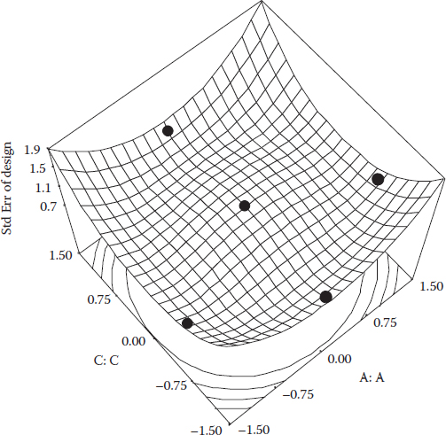
For a design with a better balance, consider another sort of SCD called the “hybrid” (Roquemore, 1976). These minimal-run (or nearly so) second-order designs for 3, 4, 6, and 7 factors resemble a standard CCD for all but the last (kth) factor, which gets set according to model-optimality criterion. Montgomery et al. (2016, p. 458) say, “It has been our experience that hybrid designs are not used as much in industrial applications as they should be… because of the ‘messy levels’ required of the extra design variable.” For example, notice the odd spread of points within the range of factor C on the standard error plot pictured in Figure 8B.1 for the three-factor hybrid design.

Table 8B.1 Number of Runs by Factor for Various Composite Designs

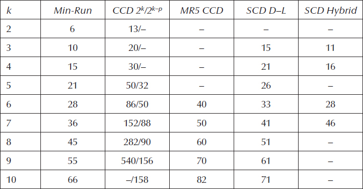
Figure 8B.1 Standard error plot for a hybrid design.

You’d best assign to this letter, or whichever comes last, the factor you find easiest to change in your process. Furthermore, we strongly advise that you add at least two additional CPs to hybrid designs—more for experiments on six or seven factors.

Templates for hybrid, D–L, and other types of SCDs are available via the Internet (Block and Mee). Many of them are encoded in RSM software such as Design-Expert from Stat-Ease, Inc.

Good Alternative to SCDs: Minimum-Run Resolution V CCDs

As a general rule, you get what you pay for with SCDs that are saturated with factors, or nearly so. Therefore, no matter which flavor of SCD you choose, D–L or hybrid, every run counts; so, these designs become extremely susceptible to outliers and outright failures that cause missing data.

We suggest a more-robust alternative called “Minimum-Run Resolution V [MR5] CCD” (Oehlert and Whitcomb, 2002), which as shown in Table 8B.1, requires fewer runs than standard CCDs, but does not shave so close to the bone as the SCDs.

The MR5 CCDs feature cores of irregularly fractionated two-level factorials that are

  Equireplicated (the same number of plus and minus 1’s for each factor)

  Minimum-run (or plus 1 for equireplication) resolution V

They are provided for as many as 50 factors by the software accompanying this book. However, even with the minimal-run core, this 50-factor MR5 CCD requires 1382 runs. That may be doable, though, provided a robotic apparatus for the experimentation, or it being done only on a virtual basis, that is, via a computer simulation.

WHERE SHOULD STAR POINTS BE LOCATED FOR SMALLER-RUN CCDs?

Haven’t you had enough of this yet? Fortunately, we need not open up another can of worms on how to set the alpha levels: Apply the same considerations for SCDs and MR5 CCDs as you would for any other CCD—that is, properties of rotatability, orthogonality of blocks, etc.