Practical Aspects for RSM Success
Keep on going and the chances are you will stumble on something, perhaps when you are least expecting it. I have never heard of anyone stumbling on something sitting down.
Charles Kettering
American engineer and the holder of 186 patents
In this last chapter, you may very well stumble across a practical aspect on RSM that will put you over the top for your optimization goals. Here, we finish off our book with vital tools for handling hard-to-change (HTC) factors, right sizing your RSM design, and how to confirm your outstanding results.
Split Plots to Handle HTC Factors
As we detailed in the third edition of DOE Simplified (2015) in a new chapter (11) devoted to this topic, experimental factors often cannot be randomized easily. Split plot designs then become attractive by grouping HTC factors, albeit with a loss in power (Anderson and Whitcomb, 2014). While split plots for factorial experiments go back to nearly a century (Fisher, 1925), application of these restricted-randomization designs to RSM is a relatively recent development, finding use, for example, in wind tunnel testing, where some factors, such as wing-tip height, cannot be changed easily (English, 2007).
The details on the design and analysis of RSM split plot experiments goes beyond the scope of this book (refer to Vining et al., 2005). However, to provide an idea of how such a design comes together, let’s go back to the trebuchet case from Chapter 5. There, we reported the results of an experiment on three factors—arm length, counterweight, and missile weight—on projectile distance. It turns out, as reported by the PBS show Nova (www.pbs.org/wgbh/nova/lostempires/trebuchet/wheels.html), that “trebs” on wheels fire a lot further than the ones that remain stationary. This is purely a matter of physics as we spelled out in our note on the “Physics of the trebuchet” in Chapter 5.
MARCO POLO MISSES THE MARK BY NOT PUTTING WHEELS ON HIS TREBUCHET
The producers of the 2014 Netflix/Weinstein series Marco Polo built trebuchets that threw a 25-kilogram sandbag almost 300 meters. As you can see from the YouTube video posted at www.youtube.com/watch?v=F8xW-LkFq6A, these were not mounted on wheels, which might have added another 100 meters (33%) to the distance according to one source (www.midi-france.info/medievalwarfare/121343_perriers.htm).
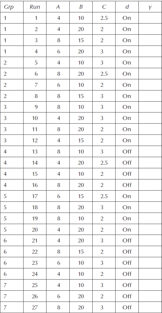
Consider a “thought experiment” on the machine pictured in Figure 5.2 where we add a fourth factor—wheels on or off. It would be very inconvenient to randomly install these or remove them between each throw. Thus, a split plot that groups firings of the trebuchet with or without wheels would be a very convenient way to accomplish this experiment. Table 12.1 lays out an optimal design with wheels being the grouped (“Grp”) HTC factor “d” (changing the case to differentiate from the easy-to-change factors randomized within groups).
By its grouping on column “d,” this 32-run split plot design provides a practical way for quantifying the effects of putting wheels on the trebuchet. Now, according to the randomized test plan, they only need to be changed every four runs—not one by one.
Table 12.1 Optimal Split Plot Design on Trebuchet
RESET HTC FACTOR(S) BETWEEN GROUPS!
When you hit the double lines drawn between groups, stop everything and see what is called for next on the HTC factors. If any or all do not change, it will be tempting to just leave them as they are. However, to generate a true measure of error that includes variation from the setup, you must reset all HTC factors, for example, take the wheels off and put them back on.
Ideally, the reset should be done from the ground up. However, when this is completely impractical, do the best you can to break the continuity of the HTC setting. For example, for furnace temperature (a common HTC factor), it might take too long for you to let things cool back down to ambient temperature. In that case, at least, open the door, remove what was on it (such as your chocolate chip cookies), turn the dial (or reset the digital control) to another temperature, and then back to the upcoming group level (e.g., 350 degrees Fahrenheit or 175 degrees Celsius for the cookies). This can be considered sufficient to reset the system. But if you do so, note it in your report as a shortcut. Full disclosure on actual experimental procedures is vital for an accurate interpretation of results by statisticians and subject-matter experts, as well.
Right-Sizing Designs via Fraction of Design Space Plots
By sizing experiment designs properly, researchers can assure that they specify a sufficient number of runs to reveal any important effects on the system. For factorial designs, this can be done by calculating statistical power (Anderson and Whitcomb, March 2014). However, the test matrices for RSM generally do not exhibit orthogonality; thus, the effect on calculations becomes correlated and degrades the statistical power. This becomes especially troublesome for constrained designs such as the one for the experiment on the air-driven mechanical part that we illustrated in Figure 7.6.
Fortunately, there is a work-around to using power to size designs that makes use of a tool called “fraction of design space” (FDS) plot (Zahran et al., 2003). The FDS plot displays the proportion (from zero to one) of the experiment-design space falling below the PV value (specified in terms of the standard error (SE) of the mean) on the y-axis.
THREE THINGS THAT AFFECT PRECISION OF PREDICTION
When the goal is optimization (usually the case for RSM), the emphasis is on producing a precisely fitted surface. The response surface is drawn by predicting the mean outcome as a function of inputs over the region of experimentation. How precisely the surface can be fit (or the mean values estimated) is a function of the SE of the predicted mean response—the smaller the SE the better. The SE of the predicted mean response at any point in the design space is a function of three things:
1. The experimental error (expressed as a standard deviation)
2. The experiment design—then the number of runs and their location
3. Where the point is located in the design space (its coordinates)
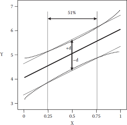
To keep things really simple for illustrating FDS plots, let’s consider fitting a straight line, the thick one shown in Figure 12.1, to response data (y) as a function of one factor (x). Naturally, as more runs are made, the more precise this fit becomes. However, due to practical limits on the run budget, it becomes necessary to be realistic in establishing the desired precision “d”—the half-width of the thin-lined interval depicted in Figure 12.1.
This simple case simulates five runs—two at each end and one in the middle of the 0–1 range—from which a CI can be calculated. The CI is displayed by the dotted lines that flare out characteristically at the extremes of the factor. Unfortunately, only 51% of the experimental region provides mean response predictions within the desired precision plus-or-minus d. This is the FDS, reported as 0.51 on a scale of zero to one. More runs, only a few in this case, are needed to push FDS above the generally acceptable level of 80%.
Figure 12.1 FDS illustrated for a simple one-factor experiment.
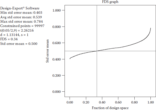
Now that you have seen what FDS measures for one factor, let’s move up by 1D to a 2D view by revisiting the case of the air-driven mechanical part. Figure 12.2 illustrates an FDS graph with the crosshair set at the level of 0.5 on the SE of the mean (y-axis). It tells us that about one-third (FDS = 0.34) of the experimental region will provide predictions within this specified SE with 95% confidence (alpha of 0.05).
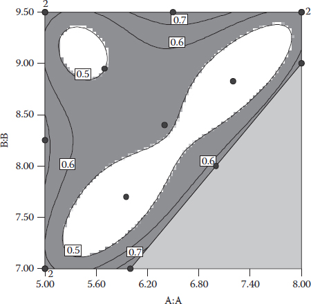
Figure 12.3, a contour plot of SE, shows which regions fall below the 0.5 level of SE.
Notice that only about a third of the triangular experimental region falls within the two areas bordered by the 0.5 SE contours. This directly corresponds to the 0.34 FDS measure. Again, look at Figure 12.3 and find the 0.6 SE contour—it falls near the perimeter of the experimental region. The FDS for 0.6 SE comes to 0.83; in other words, 83% of the experimental region can be estimated to within this level of precision.
Whether the 15-run design (the points in Figure 12.3, three of which are replicated) is sized properly depends on the ratio of the required precision “d” to the standard deviation “s.” Given software that generates FDS plots (such as the program accompanying this book), you need to only enter these two numbers to evaluate your design. In this case, let’s assume that the values for d and s are 1.5 and 1, respectively. The SE derived from this 1.5 standard-deviation requirement on precision is 0.663. (To be specific, it equals 1.5 divided by the two-tailed t-value for alpha of 0.05 with N minus p df, where N is the number of runs and p is the number of terms including the intercept.) As displayed by the FDS plot in Figure 12.4, a healthy 94% of the experiment-design space falls within this SE.
Figure 12.2 FDS illustrated for the two-factor experiment on an air-driven mechanical part.
Figure 12.3 Contour plot of SE with regions above 0.5 shaded out.
Figure 12.4 FDS based on actual requirements for RSM experiment on the air-driven mechanical system.
This far exceeds the acceptable FDS of 80%. Therefore, all systems are going to the engineer who is running this experiment.
HOW BEING PLUGGED IN ONLY TO POWER COULD OVERLOAD AN RSM EXPERIMENT
In a more detailed write-up on FDS plots for sizing the RSM experiment on the air-driven mechanical system, we calculate the price that test engineers would pay by trying to power up all the individual effect estimates (Anderson et al., 2016). The problem stems from variance inflation caused by high multiple correlation coefficients (). These indicate how much the coefficient for each individual term is correlated to the others. Ideally, all values will be zero, that is, no correlation, and thus the matrix becomes orthogonal. However, this cannot be counted on for RSM experiments. In this case, terms A, B, and AB come in at 0.778, 0.764, and 0.783 multiple correlation coefficients, respectively. To get the worst of these three estimates, AB by a hair, powered up properly to 80% for detecting a 1.5 standard-deviation effect would require more than 200 test runs. That would sink the experiment unnecessarily—given that only 15 runs suffice on the basis of the FDS sizing, as we just illustrated. So, you would at best unplug the power for assessing RSM designs.
For nonorthogonal designs, such as RSM along the lines of our example, FDS plotting works much better and more appropriately for the purpose of optimization than statistical power for “right-sizing” experiment designs. They generally lead to a smaller number of runs while providing the assurance needed that, whether or not anything emerges to be significant, the results will be statistically defensible.
Process modeling via RSM relies on empirical data and approximation by polynomial equations. As we spelled out in Chapter 2, the end result may be of no use whatsoever for prediction. Therefore, it is essential that all RSM models must be confirmed.
One approach for confirmation, which we discussed in Chapter 2, randomly splits out a subset, up to 50%, of the raw data into a validation sample. However, this works well only for datasets above a certain size (refer back to a formulaic rule of thumb) as it wastes too many runs (50% if you follow the cited protocol). A far simpler and most obvious way to confirm a model is to follow-up your experiment with one or more runs at the recommended conditions. Then, see if they fall within the 95% PI, which we detailed in Chapter 4 in the note on “Formulas for Standard Error (SE) of Predictions.”
To provide a convincing evidence of confirmation, you should replicate the confirmation run at least three times. More runs are better. However, your returns will diminish due to the PI being bounded by the CI, which is dictated by the sample size N—the number of runs in your original experiment. For example, going back to the chemical reaction case in Chapter 4, we reported that the optimal conditions produced a predicted yield of 89.1 grams with a 95% PI of 85.4–92.9 grams for a single-confirmation run (n = 1). Here is the progression of this PI for further confirmation runs:
 Three (n = 3): 86.3–92.0 grams
Six (6): 86.5–91.8 grams
Twelve (12): 86.7–91.6 grams
One million (1,000,000): 86.8–91.5 grams
The 95% CI is 86.8–91.5 grams. These are the limiting PI values as you can surmise from the interval for a million runs.
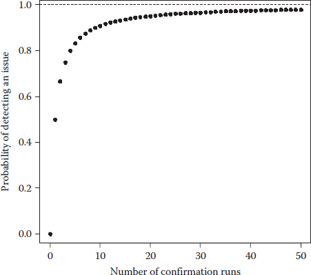
Figure 12.5 graphically lays out the probability of detecting an issue versus the number of confirmation runs (Bezener, 2015).
We recommend that at the least, you do two confirmation runs at the predicted optimum, but six or so would be nearly ideal. The best return on investment in confirmation comes with 5–10 runs. Beyond 10 runs, the investment in confirmation does not provide a good return (Jensen, 2015).
Figure 12.5 Probability of detecting an issue versus the number of confirmation runs.
PERFECTING THE RECIPE FOR RAMEN NOODLES: CASE FOR CONFIRMATION
Programmers and statisticians at Stat-Ease teamed up on an experiment to optimize the recipe for ramen noodles as a function of the amount of water, cooking time, brand, and flavor. They settled on chicken that produced great sensory results no matter what the brand, provided it was produced with just the right amount of water and cooked for an optimal time. The lead experimenter, Brooks Henderson, then produced seven bowls of ramen, three according to the perfect recipe, and four others at inferior conditions to keep the tasters honest. Happily, everything fell into place for all the measured attributes, which included not only the sensory evaluations for taste and crunchiness, but also physical changes caused by the hydration process. For example, the model predicted a weight gain of 174% for the noodles. The confirmation average (n = 3) came only to 160.2%. However, this fell well within the 95% PI of 137.3%–210.9%. This is the way to fuel technical workers, that is, provide good-quality ramen that soaks up lots of water and therefore maximizes the well-being that results from a full stomach.
Confirming the Optimal Ramen, Stat-Teaser Newsletter, January 2013, p. 3, Stat-Ease, Inc.
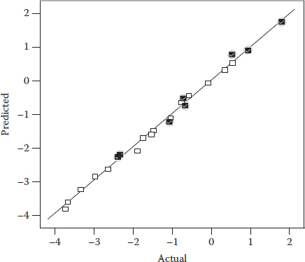
Figure 12.6 Actual versus predicted response plot included with verification points.
Another approach for confirmation is to do it concurrently, that is, during the actual experiment. This makes sense when it takes a long time to complete a block of runs and/or measure the responses. Sometimes, the opportunity for experimentation, for example, on a manufacturing scale, is limited to one shot. In these situations, it will be advantageous to embed a number of runs within your experiment design that are set aside from the others only for verification. These verification runs are added to and randomized with the DOE runs. However, they are not used to estimate the model; only the design runs are used. Then, after the experiment is completed and the results are analyzed, the predicted values of the verification runs are compared to their observed values. If they fall in line, then the model is confirmed.
Figure 12.6 shows an example where the verification points fall in line with their predicted values.
In this case, the model is clearly confirmed.
On that positive note, we conclude our primer on RSM. We hope that you will do well by applying RSM to your process—all the best!