Probability is the proportion or percentage of the time that specified things happen. The term probability is also used in reference to the art and science of determining the proportion or percentage of the time that specified things happen.
We say something is true because we’ve seen or deduced it. If we believe something is true or has taken place but we aren’t sure, it’s tempting to say it is or was “likely.” It’s wise to resist this temptation.
When people formulate a theory, they often say that something “probably” happened in the distant past, or that something “might” exist somewhere, as-yet undiscovered, at this moment. Have you ever heard that there is a “good chance” that extraterrestrial life exists? Such a statement is meaningless. Either it exists, or it does not.
If you say “I believe the universe began with an explosion,” you are stating the fact that you believe it, not the fact that it is true or that it is “probably” true. If you say “The universe began with an explosion!” your statement is logically sound, but it is a statement of a theory, not a proven fact. If you say “The universe probably started with an explosion,” you are in effect suggesting that there were multiple pasts and the universe had an explosive origin in more than half of them. This is an instance of what can be called the probability fallacy (abbreviated PF), wherein probability is injected into a discussion inappropriately.
Whatever is, is. Whatever is not, is not. Whatever was, was. Whatever was not, was not. Either the universe started with an explosion, or it didn’t. Either there is life on some other world, or there isn’t.
If we say that the “probability” of life existing elsewhere in the cosmos is 20%, we are in effect saying, “Out of n observed universes, where n is some large number, 0.2n universes have been found to have extraterrestrial life.” That doesn’t mean anything to those of us who have seen only one universe!
It is worthy of note that there are theories involving so-called fuzzy truth, in which some things “sort of happen.” These theories involve degrees of truth that span a range over which probabilities can be assigned to occurrences in the past and present. An example of this is quantum mechanics, which is concerned with the behavior of subatomic particles. Quantum mechanics can get so bizarre that some scientists say, “If you claim to understand this stuff, then you are lying.” We aren’t going to deal with anything that esoteric.
Probability is usually defined according to the results of observations, although it is sometimes defined on the basis of theory alone. When the notion of probability is abused, seemingly sound reasoning can be employed to come to absurd conclusions. This sort of thing is done in industry every day, especially when the intent is to get somebody to do something that will cause somebody else to make money. Keep your “probability fallacy radar” on when navigating through the real world.
If you come across an instance where an author (including me) says that something “probably happened,” “is probably true,” or “is likely to take place,” think of it as another way of saying that the author believes or suspects that something happened, is true, or is expected to take place on the basis of experimentation or observation.
Here are definitions of some common terms that will help us understand what we are talking about when we refer to probability.
The terms event and outcome are easily confused. An event is a single occurrence or trial in the course of an experiment. An outcome is the result of an event.
If you toss a coin 100 times, there are 100 separate events. Each event is a single toss of the coin. If you throw a pair of dice simultaneously 50 times, each act of throwing the pair is an event, so there are 50 events.
Suppose, in the process of tossing coins, you assign “heads” a value of 1 and “tails” a value of 0. Then when you toss a coin and it comes up “heads,” you can say that the outcome of that event is 1. If you throw a pair of dice and get a sum total of 7, then the outcome of that event is 7.
The outcome of an event depends on the nature of the hardware and processes involved in the experiment. The use of a pair of “weighted” dice usually produces different outcomes, for an identical set of events, than a pair of “unweighted” dice. The outcome of an event also depends on how the event is defined. There is a difference between saying that the sum is 7 in a toss of two dice, as compared with saying that one of the die comes up 2 while the other one comes up 5.
A sample space is the set of all possible outcomes in the course of an experiment. Even if the number of events is small, a sample space can be large.
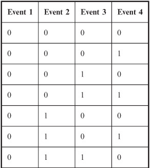
Table 8-1 The sample space for an experiment in which a coin is tossed four times. There are 16 possible outcomes; “heads” = 1 and “tails” = 0.

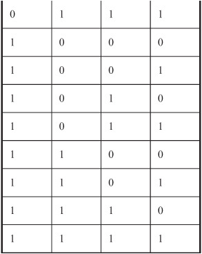
If you toss a coin four times, there are 16 possible outcomes. These are listed in Table 8-1, where “heads” = 1 and “tails” = 0. (If the coin happens to land on its edge, you disregard that result and toss it again.)
If a pair of dice, one red and one blue, is tossed once, there are 36 possible outcomes in the sample space, as shown in Table 8-2. The outcomes are
Table 8-2 The sample space for an experiment consisting of a single event, in which a pair of dice (one red, one blue) is tossed once. There are 36 possible outcomes, shown as ordered pairs (red, blue).
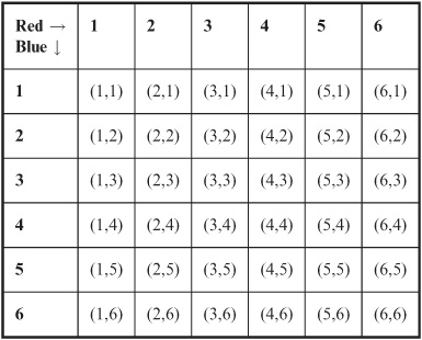
denoted as ordered pairs, with the face-number of the red die listed first and the face-number of the blue die listed second.
Let x be a discrete random variable that can attain n possible values, all equally likely. Suppose an outcome H results from exactly m different values of x, where m ≤ n. Then the mathematical probability pmath(H) that outcome H will result from any given value of x is given by the following formula:
pmath(H) = m/n
Expressed as a percentage, the probability p%(H) is:
pmath%(H) = 100m/n
If we toss an “unweighted” die once, each of the six faces is as likely to turn up as each of the others. That is, we are as likely to see 1 as we are to see 2, 3, 4, 5, or 6. In this case, there are 6 possible values, so n = 6. The mathematical probability of any one of the faces turning up (m = 1) is equal to pmath(H) = 1/6. To calculate the mathematical probability of either of any two different faces turning up (say 3 or 5), we set m = 2; therefore pmath(H) = 2/6 = 1/3. If we want to know the mathematical probability that any one of the six faces will turn up, we set m = 6, so the formula gives us pmath(H) = 6/6 = 1. The respective percentages pmath%(H) in these cases are 16.67% (approximately), 33.33% (approximately), and 100% (exactly).
Mathematical probabilities can only exist within the range 0 to 1 (or 0% to 100%) inclusive. The following formulas describe this constraint:
0 ≤ pmath(H) ≤ 1
0% ≤ pmath%(H) ≤ 100%
We can never have a mathematical probability of 2, or –45%, or –6, or 556%. When you give this some thought, it is obvious. There is no way for something to happen less often than never. It’s also impossible for something to happen more often than all the time.
In order to determine the likelihood that an event will have a certain outcome in real life, we must rely on the results of prior experiments. The chance of something happening based on experience or observation is called empirical probability.
Suppose we are told that a die is “unweighted.” How does the person who tells us this know that it is true? If we want to use this die in some application, such as when we need an object that can help us to generate a string of random numbers from the set {1, 2, 3, 4, 5, 6}, we can’t take on faith the notion that the die is “unweighted.” We have to check it out. We can analyze the die in a lab and figure out where its center of gravity is; we measure how deep the indentations are where the dots on its faces are inked. We can scan the die electronically, X-ray it, and submerge it in (or float it on) water. But to be absolutely certain that the die is “unweighted,” we must toss it many thousands of times, and be sure that each face turns up, on the average, 1/6 of the time. We must conduct an experiment – gather empirical evidence – that supports the contention that the die is “unweighted.” Empirical probability is based on determinations of relative frequency, which was discussed in the last chapter.
As with mathematical probability, there are limits to the range an empirical probability figure can attain. If H is an outcome for a particular single event, and the empirical probability of H taking place as a result of that event is denoted pemp(H), then:
0 ≤ pemp(H) ≤ 1
0% ≤ pemp%(H) ≤ 100%
Suppose a new cholesterol-lowering drug comes on the market. If the drug is to be approved by the government for public use, it must be shown effective, and it must also be shown not to have too many serious side effects. So it is tested. During the course of testing, 10,000 people, all of whom have been diagnosed with high cholesterol, are given this drug. Imagine that 7289 of the people experience a significant drop in cholesterol. Also suppose that 307 of these people experience adverse side effects. If you have high cholesterol and go on this drug, what is the empirical probability pemp(B) that you will derive benefit? What is the empirical probability pemp(A) that you will experience adverse side effects?
Some readers will say that this question cannot be satisfactorily answered because the experiment is not good enough. Is 10,000 test subjects a large enough number? What physiological factors affect the way the drug works? How about blood type, for example? Ethnicity? Gender? Blood pressure? Diet? What constitutes “high cholesterol”? What constitutes a “significant drop” in cholesterol level? What is an “adverse side effect”? What is the standard drug dose? How long must the drug be taken in order to know if it works? For convenience, we ignore all of these factors here, even though, in a true scientific experiment, it would be an excellent idea to take them all into consideration.
Based on the above experimental data, shallow as it is, the relative frequency of effectiveness is 7289/10,000 = 0.7289 = 72.89%. The relative frequency of ill effects is 307/10,000 = 0.0307 = 3.07%. We can round these off to 73% and 3%. These are the empirical probabilities that you will derive benefit, or experience adverse effects, if you take this drug in the hope of lowering your high cholesterol. Of course, once you actually use the drug, these probabilities will lose all their meaning for you. You will eventually say “The drug worked for me” or “The drug did not work for me.” You will say, “I had bad side effects” or “I did not have bad side effects.”
Empirical probability is used by scientists to make predictions. It is not good for looking at aspects of the past or present. If you try to calculate the empirical probability of the existence of extraterrestrial life in our galaxy, you can play around with formulas based on expert opinions, but once you state a numeric figure, you commit the PF. If you say the empirical probability that a hurricane of category 3 or stronger struck the US mainland in 1992 equals x% (where x < 100) because at least one hurricane of that intensity hit the US mainland in x of the years in the 20th century, historians will tell you that is rubbish, as will anyone who was in Homestead, Florida on August 24, 1992.
Imperfection is inevitable in the real world. We can’t observe an infinite number of people and take into account every possible factor in a drug test. We cannot toss a die an infinite number of times. The best we can hope for is an empirical probability figure that gets closer and closer to the “absolute truth” as we conduct a better and better experiment. Nothing we can conclude about the future is a “totally sure bet.”
Here are some formulas that describe properties of outcomes in various types of situations. Don’t let the symbology intimidate you. It is all based on the set theory notation covered in Chapter 1.
Suppose you toss an “unweighted” die many times. You get numbers turning up, apparently at random, from the set {1, 2, 3, 4, 5, 6}. What will the average value be? For example, if you toss the die 100 times, total up the numbers on the faces, and then divide by 100, what will you get? Call this number d (for die). It is reasonable to suppose that d will be fairly close to the mean, μ:
d ≈ μ
d ≈ (1 + 2 + 3 + 4 + 5 + 6)/6
= 21/6
= 3.5
It’s possible, in fact likely, that if you toss a die 100 times you’ll get a value of d that is slightly more or less than 3.5. This is to be expected because of “reality imperfection.” But now imagine tossing the die 1000 times, or 100,000 times, or even 100,000,000 times! The “reality imperfections” will be smoothed out by the fact that the number of tosses is so huge. The value of d will converge to 3.5. As the number of tosses increases without limit, the value of d will get closer and closer to 3.5, because the opportunity for repeated coincidences biasing the result will get smaller and smaller.
The foregoing scenario is an example of the law of large numbers. In a general, informal way, it can be stated like this: “As the number of events in an experiment increases, the average value of the outcome approaches the mean.” This is one of the most important laws in all of probability theory.
Two outcomes H1 and H2 are independent if and only if the occurrence of one does not affect the probability that the other will occur. We write it this way:
p(H1 ∩ H2)= p(H1)p(H2)
Figure 8-1 illustrates this situation in the form of a Venn diagram. The intersection is shown by the darkly shaded region.
A good example of independent outcomes is the tossing of a penny and a nickel. The face (“heads” or “tails”) that turns up on the penny has no effect on the face (“heads” or “tails”) that turns up on the nickel. It does not matter whether the two coins are tossed at the same time or at different times. They never interact with each other.
To illustrate how the above formula works in this situation, let p(P) represent the probability that the penny turns up “heads” when a penny and a nickel are both tossed once. Clearly, p(P) = 0.5 (1 in 2). Let p(N) represent the probability that the nickel turns up “heads” in the same scenario. It’s obvious that p(N) = 0.5 (also 1 in 2). The probability that both coins turn up “heads” is, as you should be able to guess, 1 in 4, or 0.25. The above formula states it this way, where the intersection symbol ∩ can be translated as “and”:
p(P ∩ N) = p(P)p(N)
= 0.5 × 0.5
= 0.25
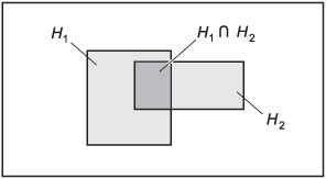
Fig. 8-1. Venn diagram showing intersection.
Let H1 and H2 be two outcomes that are mutually exclusive; that is, they have no elements in common:
H1 ∩ H2 = Ø
In this type of situation, the probability of either outcome occurring is equal to the sum of their individual probabilities. Here’s how we write it, with the union symbol ∪ translated as “either/or”:
p(H1 ∪ H2) = p(H1) + p(H2)
Figure 8-2 shows this as a Venn diagram.
When two outcomes are mutually exclusive, they cannot both occur. A good example is the tossing of a single coin. It’s impossible for “heads” and “tails” to both turn up on a given toss. But the sum of the two probabilities (0.5 for “heads” and 0.5 for “tails” if the coin is “balanced”) is equal to the probability (1) that one or the other outcome will take place.
Another example is the result of a properly run, uncomplicated election for a political office between two candidates. Let’s call the candidates Mrs. Anderson and Mr. Boyd. If Mrs. Anderson wins, we get outcome A, and if Mr. Boyd wins, we get outcome B. Let’s call the respective probabilities of their winning p(A) and p(B). We might argue about the actual values of p(A) and p(B). We might obtain empirical probability figures by conducting a poll prior to the election, and get the idea that pemp(A) = 0.29 and pemp(B) = 0.71. The probability that either Mrs. Anderson or Mr. Boyd will win is equal to the sum of p(A) and p(B), whatever these values happen to be, and we can be sure it is equal to 1 (assuming neither of the candidates quits during the election and is replaced by a third, unknown person, and assuming there
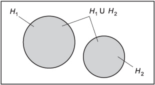
Fig. 8-2. Venn diagram showing a pair of mutually exclusive outcomes.
are no write-ins or other election irregularities). Mathematically:
p(A ∪ B) = p(A) + p(B)
= pemp(A) + pemp(B)
= 0.29 + 0.71
= 1
If two outcomes H1 and H2 are complementary, then the probability, expressed as a ratio, of one outcome is equal to 1 minus the probability, expressed as a ratio, of the other outcome. The following equations hold:
p(H2) = 1 – p(H1)
p(H1) = 1 – p(H2)
Expressed as percentages:
p%(H2) = 100 – p%(H1)
p%(H1) = 100 – p%(H2)
Figure 8-3 shows this as a Venn diagram.
The notion of complementary outcomes is useful when we want to find the probability that an outcome will fail to occur. Consider again the election between Mrs. Anderson and Mr. Boyd. Imagine that you are one of those peculiar voters who call themselves “contrarians,” and who vote against, rather than for, candidates in elections. You are interested in the probability
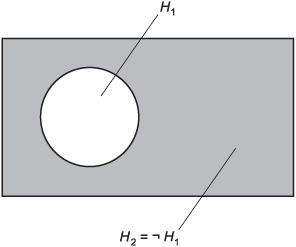
Fig. 8-3. Venn diagram showing a pair of complementary outcomes.
that “your candidate” (the one you dislike more) will lose. According to the pre-election poll, pemp(A) = 0.29 and pemp(B) = 0.71. We might state this inside-out as:
Pemp(¬B) = 1 – pemp(B)
= 1 – 0.71
= 0.29
pemp(¬A) = 1 – Pemp(A)
= 1 – 0.29
= 0.71
where the “droopy minus sign” (¬) stands for the “not” operation, also called logical negation. If you are fervently wishing for Mr. Boyd to lose, then you can guess from the poll that the likelihood of your being happy after the election is equal to pemp(¬B), which is 0.29 in this case.
Note that in order for two outcomes to be complementary, the sum of their probabilities must be equal to 1. This means that one or the other (but not both) of the two outcomes must take place; they are the only two possible outcomes in a scenario.
Outcomes H1 and H2 are called nondisjoint if and only if they have at least one element in common:
H1 ∩ H2 ≠ Ø
In this sort of case, the probability of either outcome is equal to the sum of the probabilities of their occurring separately, minus the probability of their occurring simultaneously. The equation looks like this:
p(H1 ∪ H2) = p(H1) + p(H2) – p(H1 ∩ H2)
Figure 8-4 shows this as a Venn diagram. The intersection of probabilities is subtracted in order to ensure that the elements common to both sets (represented by the lightly shaded region where the two sets overlap) are counted only once.
Imagine that a certain high school has 1000 students. The new swimming and diving coach, during his first day on the job, is looking for team prospects.
Fig. 8-4. Venn diagram showing a pair of nondisjoint outcomes.
Suppose that the following are true:
• 200 students can swim well enough to make the swimming team
• 100 students can dive well enough to make the diving team
• 30 students can make either team or both teams
If the coach wanders through the hallways blindfolded and picks a student at random, determine the probabilities, expressed as ratios, that the coach will pick
• a fast swimmer; call this p(S)
• a good diver; call this p(D)
• someone good at both swimming and diving; call this p(S ∩ D)
• someone good at either swimming or diving, or both; call this p(S ∪ D)
This problem is a little tricky. We assume that the coach has objective criteria for evaluating prospective candidates for his teams! That having been said, we must note that the outcomes are not mutually exclusive, nor are they independent. There is overlap, and there is interaction. We can find the first three answers immediately, because we are told the numbers:
p(S) = 200/1000 = 0.200
p(D) = 100/1000 = 0.100
p(S ∩ D) = 30/1000 = 0.030
In order to calculate the last answer – the total number of students who can make either team or both teams – we must find p(S ∪ D) using this formula:
p(S ∪ D) = p(S) + p(D) = p(S ∩ D)
= 0.200 + 0.100 – 0.030
= 0.270
This means that 270 of the students in the school are potential candidates for either or both teams. The answer is not 300, as one might at first expect. That would be the case only if there were no students good enough to make both teams. We mustn’t count the exceptional students twice. (However well somebody can act like a porpoise, he or she is nevertheless only one person!)
The formulas for determining the probabilities of mutually exclusive and nondisjoint outcomes can be extended to situations in which there are three possible outcomes.
Three mutually exclusive outcomes. Let H1, H2, and H3 be three mutually exclusive outcomes, such that the following facts hold:
H1 ∩ H2 = Ø
H1 ∩ H3 = Ø
H2 ∩ H3 = Ø
The probability of any one of the three outcomes occurring is equal to the sum of their individual probabilities (Fig. 8-5):
p(H1 ∪ H2 ∪ H3) = p(H1) + p(H2) + p(H3)
Three nondisjoint outcomes. Let H1, H2, and H3 be three nondisjoint outcomes. This means that one or more of the following facts is true:
H1 ∪ H2 ≠ Ø
H1 ∪ H3 ≠ Ø
H2 ∪ H3 ≠ Ø
The probability of any one of the outcomes occurring is equal to the sum of the probabilities of their occurring separately, minus the probabilities of each
Fig. 8-5. Venn diagram showing three mutually exclusive outcomes.
pair occurring simultaneously, minus the probability of all three occurring simultaneously (Fig. 8-6):
p(H1 ∪ H2 ∪ H3)
= p(H1) + p(H2) + p(H3)
– p(H1 ∩ H2) – p(H1 ∩ H3 – p(H2 ∩ H3)
– p(H1 ∩ H2 ∩ H3)
Consider again the high school with 1000 students. The coach seeks people for the swimming, diving, and water polo teams in the same wandering, blindfolded way as before. Suppose the following is true of the students in the school:
• 200 people can make the swimming team
• 100 people can make the diving team
• 150 people can make the water polo team
• 30 people can make both the swimming and diving teams
• 110 people can make both the swimming and water polo teams
• 20 people can make both the diving and water polo teams
• 10 people can make all three teams
If the coach staggers around and tags students at random, what is the probability, expressed as a ratio, that the coach will, on any one tag, select a student who is good enough for at least one of the sports?
Fig. 8-6. Venn diagram showing three nondisjoint outcomes.
Let the following expressions stand for the respective probabilities, all representing the results of random selections by the coach (and all of which we are told):
• Probability that a student can swim fast enough = p(S) = 200/1000 = 0.200
• Probability that a student can dive well enough = p(D) = 100/1000 = 0.100
• Probability that a student can play water polo well enough = p(W) = 150/1000 = 0.150
• Probability that a student can swim fast enough and dive well enough = p(S ∩ D) = 30/1000 = 0.030
• Probability that a student can swim fast enough and play water polo well enough = p(S ∩ W) = 110/1000 = 0.110
• Probability that a student can dive well enough and play water polo well enough = p(D ∩ W) = 20/1000 = 0.020
• Probability that a student can swim fast enough, dive well enough, and play water polo well enough = p(S ∩ D ∩ W) = 10/1000 = 0.010
In order to calculate the total number of students who can end up playing at least one sport for this coach, we must find p(S ∪ D ∪ W) using this formula:
p(S ∪ D ∪ W) = p(S) + p(D) + p(W)
– p(S ∩ D) – p(S ∩ W) – p(D ∩ W)
– p(S ∩ D ∩ W)
= 0.200 + 0.100 + 0.150
– 0.030 – 0.110 – 0.020 – 0.010
= 0.280
This means that 280 of the students in the school are potential prospects.
In probability, it is often necessary to choose small sets from large ones, or to figure out the number of ways in which certain sets of outcomes can take place. Permutations and combinations are the two most common ways this is done.
When working with multiple possibilities, it’s necessary to be familiar with a function called the factorial. This function applies only to the natural numbers. (It can be extended to more values, but then it is called the gamma function.) The factorial of a number is indicated by writing an exclamation point after it.
If n is a natural number and n ≥ 1, the value of n! is defined as the product of all natural numbers less than or equal to n:
n! = 1 × 2 × 3 × 4 × . . . × n
If n = 0, then by convention, n! = 1. The factorial is not defined for negative numbers.
It’s easy to see that as n increases, the value of n! goes up rapidly, and when n reaches significant values, the factorial skyrockets. There is a formula for approximating n! when n is large:
n! ≈ nn/en
where e is a constant called the natural logarithm base, and is equal to approximately 2.71828. The squiggly equals sign emphasizes the fact that the value of n! using this formula is approximate, not exact.
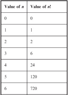
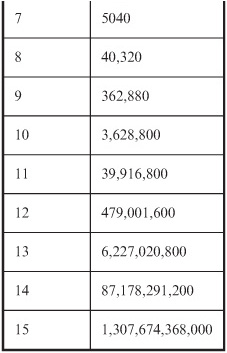
Write down the values of the factorial function for n = 0 through n = 15, in order to illustrate just how fast this value “blows up.”
The results are shown in Table 8-3. It’s perfectly all right to use a calculator here. It should be capable of displaying a lot of digits. Most personal computers have calculators that are good enough for this purpose.
Table 8-3 Values of n! for n = 0 through n = 15. This table constitutes the solution to Problem 8-4.
Determine the approximate value of 100! using the formula given above.
A calculator is not an option here; it is a requirement. You should use one that has an ex (or natural exponential) function key. In case your calculator does not have this key, the value of the exponential function can be found by using the natural logarithm key and the inverse function key together. It will also be necessary for the calculator to have an xy key (also called x^y) that lets you find the value of a number raised to its own power. In addition, the calculator should be capable of displaying numbers in scientific notation, also called power-of-10 notation. Most personal computer calculators are adequate if they are set for scientific mode.
Using the above formula for n = 100:
100! ≈ (100100)/e100
≈ (1.00 × 10200)/(2.688117 × 1043)
≈ 3.72 10156
The numeral representing this number, if written out in full, would be a string of digits too long to fit on most text pages without taking up two or more lines. Your calculator will probably display it as something like 3.72e+156 or 3.72 E 156. In these displays, the “e” or “E” does not refer to the natural logarithm base. Instead, it means “times 10 raised to the power of.”
When working with problems in which items are taken from a larger set in specific order, the idea of a permutation is useful. Suppose q and r are both positive integers. Let q represent a set of items or objects taken r at a time in a specific order. The possible number of permutations in this situation is symbolized qPr and can be calculated as follows:
qPr = q!/(q – r)!
Let q represent a set of items or objects taken r at a time in no particular order, and where both q and r are positive integers. The possible number of combinations in this situation is symbolized qCr and can be calculated as follows:
qCr = qPr/r! = q!/[r!(q – r)!]
How many permutations are there if you have 10 apples, taken 5 at a time in a specific order?
Use the above formula for permutations, plugging in q = 10 and r = 5:
10P5 = 10!/(10 – 5)!
= 10!/5!
= 10 × 9 × 8 × 7 × 6
= 30,240
How many combinations are there if you have 10 apples, taken 5 at a time in no particular order?
Use the above formula for combinations, plugging in q= 10 and r= 5. We can use the formula that derives combinations based on permutations, because we already know from the previous problem that 10P5 = 30,240:
10C5 = 10P5/5!
= 30,240/120
= 252
Refer to the text in this chapter if necessary. A good score is eight correct. Answers are in the back of the book.
1. Empirical probability is based on
(a) observation or experimentation
(b) theoretical models only
(d) standard deviations
2. What is the number of possible combinations of 7 objects taken 3 at a time?
(a) 10
(b) 21
(c) 35
(d) 210
3. What is the number of possible permutations of 7 objects taken 3 at a time?
(a) 10
(b) 21
(c) 35
(d) 210
4. The difference between permutations and combinations lies in the fact that
(a) permutations take order into account, but combinations do not
(b) combinations take order into account, but permutations do not
(c) combinations involve only continuous variables, but permutations involve only discrete variables
(d) permutations involve only continuous variables, but combinations involve only discrete variables
5. The result of an event is called
(a) an experiment
(b) a trial
(c) an outcome
(d) a variable
6. How many times as large is 1,000,000 factorial, compared with 999,999 factorial?
(a) 1,000,000 times as large.
(b) 999,999 times as large.
(c) A huge number that requires either a computer or else many human-hours to calculate.
(d) There is not enough information given here to get any idea.
7. The set of all possible outcomes during the course of an experiment is called
(a) a dependent variable
(b) a random variable
(d) a sample space
8. What is the mathematical probability that a coin, tossed 10 times in a row, will come up “tails” on all 10 tosses?
(a) 1/10
(b) 1/64
(c) 1/1024
(d) 1/2048
9. Two outcomes are mutually exclusive if and only if
(a) they are nondisjoint
(b) they have no elements in common
(c) they have at least one element in common
(d) they have identical sets of outcomes
10. The probability, expressed as a percentage, of a particular occurrence can never be
(a) less than 100
(b) less than 0
(c) greater than 1
(d) anything but a whole number