10

An Ordered Probit Analysis
of Transaction Stock Prices

10.1 Introduction

VIRTUALLY ALL EMPIRICAL INVESTIGATIONS of the microstructure of securities markets require a statistical model of asset prices that can capture the salient features of price movements from one transaction to the next. For example, because there are several theories of why bid/ask spreads exist, a stochastic model for prices is a prerequisite to empirically decomposing observed spreads into components due to order-processing costs, adverse selection, and specialist market power.¹ The benefits and costs of particular aspects of a market's microstructure, such as margin requirements, the degree of competition faced by dealers, the frequency that orders are cleared, and intraday volatility also depend intimately on the particular specification of price dynamics.² Even the event study, a tool that does not explicitly assume any particular theory of the market microstructure, depends heavily on price dynamics (see, for example, Barclay and Litzenberger (1988)). In fact, it is difficult to imagine an economically relevant feature of transaction prices and the market microstructure that does not hinge on such price dynamics.

Since stock prices are perhaps the most closely watched economic variables to date, they have been modeled by many competing specifications, beginning with the simple random walk or Brownian motion. However, the majority of these specifications have been unable to capture at least three aspects of transaction prices. First, on most U.S. stock exchanges, prices are quoted in increments of eighths of a dollar, a feature not captured by stochastic processes with continuous state spaces. Of course, discreteness is less problematic for coarser-sampled data, which may be well-approximated by a continuousstate process. But discreteness is of paramount importance for intraday price movements, since such finely-sampled price changes may take on only five or six distinct values³.

The second distinguishing feature of transaction prices is their timing, which is irregular and random. Therefore, such prices may be modeled by discrete-time processes only if we are prepared to ignore the information contained in waiting times between trades.

Finally, although many studies have computed correlations between transaction price changes and other economic variables, to date none of the existing models of discrete transaction prices have been able to quantify such effects formally. Such models have focused primarily on the unconditional distribution of price changes, whereas what is more often of economic interest is the conditional distribution, conditioned on quantities such as volume, time between trades, and the sequence of past price changes.⁴ For example, one of the unresolved empirical issues in this literature is what the total costs of immediate execution are, which many take to be a measure of market liquidity. Indeed, the largest component of these costs may be the price impact of large trades. A floor broker seeking to unload 100,000 shares of stock will generally break up the sale into smaller blocks to minimize the price impact of the trades. How do we measure price impact? Such a question is a question about the conditional distribution of price changes, conditional upon a particular sequence of volume and price changes, i.e., order flow.

In this chapter, we propose a specification of transaction price changes that addresses all three of these issues, and yet is still tractable enough to permit estimation via standard techniques. This specification is known as ordered probit, a technique used most frequently in cross-sectional studies of dependent variables that take on only a finite number of values possessing a natural ordering.⁵ For example, the dependent variable might be the level of education, as measured by three categories: less than high school, high school, and college education. The dependent variable is discrete, and is naturally ordered since college education always follows high school (see Maddala (1983) for further details). Heuristically, ordered probit analysis is a generalization of the linear regression model to cases where the dependent variable is discrete. As such, among the existing models of stock price discreteness (e.g., Ball (1988), Cho and Frees (1988), Gottlieb and Kalay (1985), and Harris (1991)), ordered probit is perhaps the only specification that can easily capture the impact of “explanatory” variables on price changes while also accounting for price discreteness and irregular trade times.

Underlying the analysis is a “virtual” regression model with an unobserved continuous dependent variable Z* whose conditional mean is a linear function of observed “explanatory” variables. Although Z* is unobserved, it is related to an observable discrete random variable Z, whose realizations are determined by where Z* lies in its domain or state space. By partitioning the state space into a finite number of distinct regions, Z may be viewed as an indicator function for Z* over these regions. For example, a discrete random variable Z taking on the values {-,0,} may be modeled as an indicator variable that takes on the value - whenever Z* ≤ α₁,the value 0 whenever α₁ < Z* ≤ α₂, and the value whenever Z*>α₂. Ordered probit analysis consists of estimating α₁,α₂ and the coefficients of the unobserved regression model that determines the conditional mean and variance of Z*.

Since α₁,α₂, and Z* may depend on a vector of “regressors” X, ordered probit analysis is considerably more general than its simple structure suggests. In fact, it is well-known that ordered probit can fit any arbitrary multinomial distribution. However, because of the underlying linear regression framework, ordered probit can also capture the price effects of many economic variables in a way that models of the unconditional distribution of price changes cannot.

To motivate our methodology and to focus it on specific market microstructure applications, we consider three questions concerning the behavior of transaction prices. First, how does the particular sequence of trades affect the conditional distribution of price changes, and how do these effects differ across stocks? For example, does a sequence of three consecutive buyer-initiated trades (“buys”) generate price pressure, so that the next price change is more likely to be positive than if the sequence were three consecutive seller-initiated trades (“sells”), and how does this pressure change from stock to stock? Second, does trade size affect price changes as some theories suggest, and if so, what is the price impact per unit volume of trade from one transaction to the next? Third, does price discreteness matter? In particular, can the conditional distribution of price changes be modeled as a simple linear regression of price changes on explanatory variables without accounting for discreteness at all? Within the context of the ordered probit framework, we shall obtain sharp answers to each of these questions.

In Section 10.2, we review the ordered probit model and describe its estimation via maximum likelihood. We describe the data in Section 10.3 by presenting detailed summary statistics for an initial sample of six stocks. In Section 10.4, we discuss the empirical specification of the ordered probit model and the selection of conditioning or “explanatory” variables. The maximum likelihood estimates for our initial sample are reported in Section 10.5, along with some diagnostic specification tests. In Section 10.6, we use these maximum likelihood estimates in three specific applications: (1) testing for order-flow dependence, (2) measuring price impact, and (3) comparing ordered probit to simple linear regression. And as a check on the robustness of our findings, in Section 10.7 we present less detailed results for a larger and randomly chosen sample of 100 stocks. We conclude in Section 10.8.

10.2 The Ordered Probit Model

Consider a sequence of transaction prices P(to), P(t1), …, P(t_n) observed at times t₁ t₂ t₃.…,tn, and denote by Z₁, Z₂,…, Z_n the corresponding price changes, where Z_k ≡ P(t_k)-P(t_k-1) is assumed to be an integer multiple of some divisor called a “tick” (such as an eighth of a dollar). Let Z*_k denote an unobservable continuous random variable such that

where “i.n.i.d.” indicates that the ’s are independently but not identically distributed, and X _k is a q × 1 vector of predetermined variables that governs the conditional mean of Z*_k. Note that subscripts are used to denote “transaction” time, whereas time arguments t_k denote calendar or “clock” time, a convention we shall follow throughout the chapter.

The essence of the ordered probit model is the assumption that observed price changes Z_k are related to the continuous variable Z*_k in the following manner:

where the sets A_j form apartition of the state spaceS* of Z*_k, i.e., S* =U^m_j=l and A_i ∩ A_j=for i ≠ j, and the s_j’s are the discrete values that comprise the state space S of Z*_k.

The motivation for the ordered probit specification is to uncover the mapping between S* and S and relate it to a set of economic variables or “regressors.” In our current application, the s_j’s are 0, and so on, and for simplicity we define the state-space partition of S* to be intervals:

Although the observed price change can be any number of ticks, positive or negative, we assume that m in (10.2.2) is finite to keep the number of unknown parameters finite. This poses no problems, since we may always let some states in S represent a multiple (and possibly countably infinite) number of values for the observed price change. For example, in our empirical application we define s₁ to be a price change of -4 ticks or less, s₉ to be a price change of +4 ticks or more, and s₂ to s₈ to be price changes of -3 ticks to +3 ticks respectively. This parsimony is obtained at the cost of losing price resolution—under this specification the ordered probit model does not distinguish between price changes of +4 and price changes greater than +4 (since the +4tick outcome and the greater than +4tick outcome have been grouped together into a common event), and similarly for price changes of -4 ticks versus price changes less than -4. Of course, in principle the resolution may be made arbitrarily finer by simply introducing more states, i.e., by increasing m. Moreover, as long as (10.2.1) is correctly specified, then increasing price resolution will not affect the estimated β’s asymptotically (although finite sample properties may differ). However, in practice the data will impose a limit on the fineness of price resolution simply because there will be no observations in the extreme states when m is too large, in which case a subset of the parameters is not identified and cannot be estimated.

Observe that the ’s in (10.2.1) are assumed to be conditionally independently but not identically distributed, conditioned on the X_k's and other economic variables W_k influencing the conditional variance ⁶ This allows for clock-time effects, as in the case of an arithmetic Brownian motion where the variance of price changes is linear in the time between trades. We also allow for more general forms of conditional heteroskedasticity by letting depend linearly on other economic variables W_k, which differs from Engle's (1982) ARCH process only in its application to a discrete dependent variable model requiring an additional identification assumption that we shall discuss below in Section 10.4.

The dependence structure of the observed process Z_k is clearly induced by that of Z*_k and the definitions of the A_j's, since

As a consequence, if the variables X_k and W_k are temporally independent, the observed process Z_k is also temporally independent. Of course, these are fairly restrictive assumptions and are certainly not necessary for any of the statistical inferences that follow. We require only that the 's be conditionally independent, so that all serial dependence is captured by the X_k's and the W_k's. Consequently, the independence of the 's does not imply that the Z*_k’s are independently distributed because we have placed no restrictions on the temporal dependence of the X_k's or W_k' s.

The conditional distribution of observed price changes Z*_k, conditioned on X_k and W_k, is determined by the partition boundaries and the particular distribution of For Gaussian 's, the conditional distribution is

where Φ(•) is the standard normal cumulative distribution function.

To develop some intuition for the ordered probit model, observe that the probability of any particular observed price change is determined by where the conditional mean lies relative to the partition boundaries. Therefore, for a given conditional mean X'_kß, shifting the boundaries will alter the probabilities of observing each state (see Figure 10.1). In fact, by shifting the boundaries appropriately, ordered probit can fit any arbitrary multinomial distribution. This implies that the assumption of normality underlying ordered probit plays no special role in determining the probabilities of states; a logistic distribution, for example, could have served equally well.

Figure 10.1. Illustration of ordered probit pro babilities p_i of observing a price change of S_i ticks, which are determined by where the unobservable “virtual” price change Z*_k falls. In particular, if Z*_k falls in the interval (α_i-1,α_i] then the ordered probit model implies that the observed price change Z_k is s_i ticks. More formally, p_i ≡ Prob(Z*_k = s_i | X_k, W_k) = Prob(α_i-1≤α_i | X_k, W_k), i = 1,…, 9, where, for notational simplicity, we define α₀=-∞ and α₉≡+∞. The ordered probit model captures the effect of economic variables X_k, W_k on the virtual price change and places enough structure on the probabilities p_i to permit their estimation by maximum likelihood.

However, since it is considerably more difficult to capture conditional heteroskedasticity in the ordered logit model, we have chosen the Gaussian specification.

Given the partition boundaries, a higher conditional mean X'_kß implies a higher probability of observing a more extreme positive state. Of course, the labeling of states is arbitrary, but the ordered probit model makes use of the natural ordering of the states. The regressors allow us to separate the effects of various economic factors that influence the likelihood of one state versus another. For example, suppose that a large positive value of X₁ usually implies a large negative observed price change and vice versa. Then the ordered probit coefficient ß₁ will be negative in sign and large in magnitude (relative to σ_k of course).

By allowing the data to determine the partition boundaries α, the coefficients ß of the conditional mean, and the conditional variance σ_k², the ordered probit model captures the empirical relation between the unobservable continuous state space S* and the observed discrete state space S as a function of the economic variables X_k and W_k

10.2.1 Other Models of Discreteness

From these observations, it is apparent that the rounding/eighths-barriers models of discreteness in Ball (1988), Cho and Frees (1988), Gottlieb and Kalay (1985) and Harris (1991) may be reparametrized as ordered probit models. Consider first the case of a “true” price process that is an arithmetic Brownian motion, with trades occurring only when this continuous-state process crosses an eighths threshold (see Cho and Frees (1988)). Observed trades from such a process may be generated by an ordered probit model in which the partition boundaries are fixed at multiples of eighths and the single regressor is the time interval (or first-passage time) between crossings, appearing in both the conditional mean and variance of Z*_k.

To obtain the rounding models of Ball (1988), Gottlieb and Kalay (1985), and Harris (1991), which do not make use of waiting times between trades, define the partition boundaries as the midpoint between eighths, e.g., the observed price change is if the virtual price process lies in the interval and omit the waiting time as a regressor in both the conditional mean and variance (see the discussion in Section 10.6.3 below).

The generality of the ordered probit model comes from the fact that the rounding and eighths-barrier models of discreteness are both special cases of ordered probit under appropriate restrictions on the partition boundaries. In fact, since the boundaries may be parametrized to be time- and statedependent, ordered probit can allow for considerably more general kinds of rounding and eighths barriers. In addition to fitting any arbitrary multinomial distribution, ordered probit may also accommodate finite-state Markov chains and compound Poisson processes.

Of course, other models of discreteness are not necessarily obsolete, since in several cases the parameters of interest may not be simple functions of the ordered probit parameters. For example, a tedious calculation will show that although Harris's (1991) rounding model may be represented as an ordered probit model, the bid/ask spread parameter c is not easily recoverable from the ordered probit parameters. In such cases, other equivalent specifications may allow more direct estimation of the parameters of interest.

10.2.2 The Likelihood Function

Let Y_ik be an indicator variable which takes on the value one if the realization of the kth observation Z_k is the ith state s_i, and zero otherwise. Then the log-likelihood function for the vector of price changes Z=[Z₁ Z₂…Z_n]', conditional on the explanatory variables X = [X₁ X₂…X_n]', is given by

Recall that is a conditional variance, conditioned upon X_k. This allows for conditional heteroskedasticity in the Z*_k's, as in the rounding model of Cho and Frees (1988) where the Z*_k's are increments of arithmetic Brownian motion with variance proportional to t_k – t_k-1. In fact, arithmetic Brownian motion may be accommodated explicitly by the specification

More generally, we may also let depend on other economic variables W_k, so that

There are, however, some constraints that must be placed on these parameters to achieve identification since, for example, doubling the α's, the β's, and σ_k leaves the likelihood unchanged. We shall return to this issue in Section 10.4.

10.3 The Data

The Institute for the Study of Securities Markets (ISSM) transaction database consists of time-stamped trades (to the nearest second), trade size, and bid/ask quotes from the New York and American Stock Exchanges and the consolidated regional exchanges from january 4 to December 30 of 1988. Because of the sheer size of the ISSM database, most empirical studies of the market microstructure have concentrated on more manageable subsets of the database, and we also follow this practice. But because there is so much data, the “pretest” or “data-snooping” biases associated with any nonrandom selection procedure used to obtain the smaller subsets are likely to be substantial. As a simple example of such a bias, suppose we choose our stocks by the seemingly innocuous requirement that they have a minimum of 100,000 trades in 1988. This rule will impart a substantial downward bias on our measures of price impact because stocks with over 100,000 trades per year are generally more liquid and, almost by definition, have smaller price impact. Therefore, how we choose our subsample of stocks may have important consequences for how our results are to be interpreted, so we shall describe our procedure in some detail here.

We first begin with an initial “test” sample containing five stocks that did not engage in any stock splits or stock dividends greater than 3 : 2 during 1988: Alcoa, Allied Signal, Boeing, DuPont, and General Motors. We restrict splits because the effects of price discreteness to be captured by our model are likely to change in important ways with dramatic shifts in the price level; by eliminating large splits we reduce the problem of large changes in the price level without screening on prices directly. (Of course, if we were interested in explaining stock splits, this procedure would obviously impart important biases in the empirical results.) We also chose these five stocks because they are relatively large and visible companies, each with a large number of trades, and therefore likely to yield accurate parameter estimates. We then performed the standard “specification searches” on these five stocks, adding, deleting, and transforming regressors to obtain a “reasonable” fit. By “reasonable” we mean primarily the convergence of the maximum likelihood estimation procedure, but it must also include Learner's (1978) kind of informal or ad hoc inferences that all empiricists engage in.

Once we obtain a specification that is “reasonable,” we estimate it without further revision for our primary sample of six new stocks, chosen to yield a representative sample with respect to industries, market value, price levels, and sample sizes. They are International Business Machines Corporation (IBM), Quantum Chemical Corporation (CUE), Foster Wheeler Corporation (FWC), Handy and Harman Company (HNH), Navistar International Corporation (NAV), and American Telephone and Telegraph Incorporated (T). (Our original primary sample consists of eleven stocks but we omitted the results for five of them to conserve space. See Hausman, Lo, and MacKinlay (1991) for the full set of results.) By using the specification derived from the test sample on stocks in this fresh sample, we seek to lessen the impact of any data-snooping biases generated by our specification searches. If, for example, our parameter estimates and subsequent inferences change dramatically in the new sample (in fact, they do not) this might be a sign that our test-sample findings were driven primarily by selection biases.

As a final check on the robustness of our specification, we estimate it for a larger sample of 100 stocks chosen randomly, and these companies are listed in Table 10.5. From this larger sample, it is apparent that our smaller six-stock sample does suffer from at least one selection bias: it is comprised of relatively well-known companies. In contrast, relatively few companies in Table 10.5 are as familiar. Despite this bias, virtually all of our empirical findings are confirmed by the larger sample. To conserve space and to focus attention on our findings, we report the complete set of summary statistics and estimation results only for the smaller sample of six stocks, and present broader and less detailed findings for the extended sample afterwards.

Of course, as long as there is cross-sectional dependence among the two samples it is impossible to eliminate such biases completely. Moreover, samples drawn from a different time period are not necessarily free from selection bias as some have suggested, due to the presence of temporal dependence. Unfortunately, nonexperimental inference is always subject to selection biases of one kind or another since specification searches are an unavoidable aspect of genuine progress in empirical research (see, for example, Lo and MacKinlay (1990b)). Even Bayesian inference, which is not as sensitive to the kinds of selection biases discussed in Leamer (1978), can be distorted in subtle ways by specification searches. Therefore, beyond our test-sample procedure, we can only alert readers to the possibility of such biases and allow them to adjust their own inferences accordingly.

10.3.1 Sample Statistics

We take as our basic time series the intraday price changes from trade to trade, and discard all overnight price changes. That the statistical properties of overnight price changes differ considerably from those of intraday price changes has been convincingly documented by several authors, most recently by Amihud and Mendelson (1987), Stoll and Whaley (1990), and Wood, McInish, and Ord (1985). Since the three market microstructure applications we are focusing on involve intraday price behavior, and overnight price changes are different enough to warrant a separate specification, we use only intraday price changes. The first and last transaction prices of each day are also discarded, since they differ systematically from other prices due to institutional features (see Amihud and Mendelson (1987) for further details).

Several other screens were imposed to eliminate “problem” trades and quotes, yielding sample sizes ranging from 3,174 trades for HNH to 206,794 trades for IBM. Specifically: (1) all trades flagged with the following ISSM condition codes were eliminated: A, C, D, O, R, and Z (see the ISSM documentation for further details concerning trade condition codes); (2) transactions exceeding 3,276,000 shares [termed “big trades” by ISSM] were also eliminated; (3) because we use three lags of price changes and three lags of five-minute returns on the S&P 500 index futures prices as explanatory variables, we do not use the first three price changes or price changes during the first 15 minutes of each day (whichever occurs later) as observations of the dependent variable; and (4) since S&P 500 futures data were not available on November 10, 11, and the first two trading hours of May 3, trades during these times were also omitted.

For some stocks, a small number of transactions occurred at prices denominated in of a dollar (non-NYSE trades). In these cases, we rounded the price randomly (up or down) to the nearest , and if necessary, also rounded the bid/ask quotes in the same direction.

Quotes implying bid/ask spreads greater than 40 ticks or flagged with the following ISSM condition codes were also eliminated: C, D, F, G, I, L, N, P, S, V, X, and Z (essentially all “BBO-1neligible” quotes; see the ISSM documentation for further details concerning the definitions of the particular trade and quote condition codes, and Eikeboom (1992) for a thorough study of the relative frequencies of these condition codes for a small subset of the ISSM database).

Since we also use bid and ask prices in our analysis, some discussion of how we matched quotes to prices is necessary. Bid/ask quotes are reported on the ISSM tape only when they are revised, hence it is natural to match each transaction price to the most recently reported quote prior to the transaction. However, Bronfman (1991), Lee and Ready (1991), and others have shown that prices of trades that precipitate quote revisions are sometimes reported with a lag, so that the order of quote revision and transaction price is reversed in official records such as the ISSM tapes. To address this issue, we match transaction prices to quotes that are set at least five seconds prior to the transaction; the evidence in Lee and Ready (1991) suggests that this will account for most of the missequencing.

To provide some intuition for this enormous dataset, we report a few summary statistics in Table 10.1. Our sample contains considerable price dispersion, with the low stock price ranging from $3.125 for NAV to $104.250 for IBM, and the high ranging from $7.875 for NAV to $129.500 for IBM. At $219 million, HNH has the smallest market capitalization in our sample, and IBM has the largest with a market value of $69.8 billion.

For our empirical analysis we also require some indicator of whether a transaction was buyer-initiated or seller-initiated. Obviously, this is a difficult task because for every trade there is always a buyer and a seller. What we are attempting to measure is which of the two parties is more anxious to consummate the trade and is therefore willing to pay for it in the form of the bid/ask spread. Perhaps the most obvious indicator is whether the transaction occurs at the ask price or at the bid price; if it is the former then the transaction is most likely a “buy,” and if it is the latter then the transaction is most likely a “sell.” Unfortunately, a large number of transactions occur at prices strictly within the bid/ask spread, so that this method for signing trades will leave the majority of trades indeterminate.

Following Blume, MacKinlay, and Terker (1989) and many others, we classify a transaction as a buy if the transaction price is higher than the mean of the prevailing bid/ask quote (the most recent quote that is set at least five seconds prior to the trade), and classify it as a sell if the price is lower. Should the price equal the mean of the prevailing bid/ask quote, we classify the trade as an “indeterminate” trade. This method yields far fewer indeterminate trades than classifying according to transactions at the bid or at the ask.

Table 10.1. Summary statistics for transaction prices and corresponding ordered probit explanatory variables of International Business Machines Corporation (IBM-206,794 trades), Quantum Chemical Corporation (CUE - 26,927 trades), Foster Wheeler Corporation (FWC - 18,199 trades), Handy and Harman Company (HNH - 3,174 trades), Navistar International Corporation (NAV - 96,127 trades), and American Telephone and Telegraph Company (T - 180,726 trades), for the period from january 4, 1988, to December 30, 1988.

¹  Computed at the beginning of the sample period.

²  Five-minute continuously compounded returns of the S&P 500 index futures price, for the contract maturing in the closest month beyond the month in which transaction k occurred, where the return corresponding to the kth transaction is computed with the futures price recorded one minute before the nearest round minute prior to t_k and the price recorded five minutes before this.

³  Takes the value 1 if the kth transaction price is greater than the average of the quoted bid and ask prices at time t_k, the value -1 if the kth transaction price is less than the average of the quoted bid and ask prices at time t_k, and 0 otherwise.

⁴  Box-Cox transformation of dollar volume multiplied by the buy/sell indicator, where the Box- Cox parameter λ is estimated jointly with the other ordered probit parameters via maximum likelihood. The Box-Cox parameter λ determines the degree of curvature that the transformation T_λ(•) exhibits in transforming dollar volume V_k before inclusion as an explanatory variable in the ordered probit specification. If λ = 1, the transformation T_λ(•) is linear, hence dollar volume enters the ordered probit model linearly. If λ = 0, the transformation is equivalent to log(•), hence the natural logarithm of dollar volume enters the ordered probit model. When λ is between 0 and 1, the curvature of T_λ(•) is between logarithmic and linear.

 

Unfortunately, little is known about the relative merits of this method of classification versus others such as the “tick test” (which classifies a transaction as a buy, a sell, or indeterminate if its price is greater than, less than, or equal to the previous transaction's price, respectively), simply because it is virtually impossible to obtain the data necessary to evaluate these alternatives. The only study we have seen is by Robinson (1988, Chapter 4.4.1, Table 19), in which he compared the tick test rule to the bid/ask mean rule for a sample of 196 block trades initiated by two major Canadian life insurance companies, and concluded that the bid/ask mean rule was considerably more accurate.

From Table 10.1 we see that 13-26% of each stock's transactions are indeterminate, and the remaining trades fall almost equally into the two remaining categories. The one exception is the smallest stock, HNH, which has more than twice as many sells as buys.

The means and standard deviations of other variables to be used in our ordered probit analysis are also given in Table 10.1. The precise definitions of these variables will be given below in Section 10.4, but briefly, Z_k is the price change between transactions k - 1 and k, t_k is the time elapsed between these trades, AB_k is the bid/ask spread prevailing at transaction k, SP500_k is the return on the S&P 500 index futures price over the five-minute period immediately preceding transaction k, IBS_k is the buy/sell indicator described above (1 for a buy, -1 for a sell, and 0 for an indeterminate trade), and T_λ(V_k) is a transformation of the dollar volume of transaction k, transformed according to the Box and Cox (1964) specification with parameter λ_i which is estimated for each stock i by maximum likelihood along with the other ordered probit parameters.

From Table 10.1 we see that for the larger stocks, trades tend to occur almost every minute on average. Of course, the smaller stocks trade less frequently, with HNH trading only once every 18 minutes on average. The median dollar volume per trade also varies considerably, ranging from $3,000 for relatively low-priced NAV to $57,375 for higher-priced IBM.

Finally, Figure 10.2 contains histograms for the price change, timebetween- trade, and dollar volume variables for the six stocks. The histograms of price changes are constructed so that the most extreme cells also include observations beyond them, i.e., the level of the histogram for the -4 tick cell reflects all price changes of -4 ticks or less, and similarly for the +4 ticks cell. Surprisingly, these price histograms are remarkably symmetric across all stocks. Also, virtually all the mass in each histogram is concentrated in five or seven cells-there are few absolute price changes of four ticks or more, which underscores the importance of discreteness in transaction prices.

Figure 10.2. Histograms of price changes, time-between-trades, and dollar volume of International Business Machines Corporation (IBM - 206,794 trades), Quantum Chemical Corporation (CUE-26,927 trades), Foster Wheeler Corporation (FWC- 18,199 trades), Handy andHarman Company (HNH - 3,174 trades), Navistar International Corporation (NAV- 96,127 trades), and American Telephone and Telegraph Company (T - 180,726 trades), for the period from fanuary 4, 1988, to December 30, 1988.

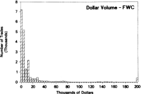
For both the time-between-trade and dollar volume variables, the largest cell, i.e., 1,500 seconds or $200,000, also includes all trades beyond it. As expected, the histograms for these quantities vary greatly according to market value and price level. For the larger stocks, the time between trades is relatively short, hence most of the mass in those histograms is in the lower- valued cells. But the histograms of smaller, less liquid stocks like HNH have spikes in the largest-valued cell. Histograms for dollar volume are sometimes bimodal, as in the case of IBM, reflecting both round-lot trading at 100 shares ($10,000 on average for IBM's stock price during 1988) and some very large trades, presumably by institutional investors.

10.4 The Empirical Specification

To estimate the parameters of the ordered probit model via maximum likelihood, we must first specify (i) the number of states m, (ii) the explanatory variables X_k and (iii) the parametrization of the variance .

In choosing m, we must balance price resolution against the practical constraint that too large an m will yield no observations in the extreme states s₁ and s_m. For example, if we set m to 101 and define the states s₁ and s₁₀₁ symmetrically to be price changes of -50 ticks and +50 ticks respectively, we would find no Z_k's among our six stocks falling into these two states. Using the histograms in Figure 10.2 as a guide, we set m = 9 for the larger stocks, implying extreme states of -4 ticks or less and +4 ticks or more. For the two smaller stocks, FWC and HNH, we set m = 5, implying extreme states of -2 ticks or less and +2 ticks or more. Although the definition of states need not be symmetric (state s₁ can be -6 ticks or less, implying that state 59 is +2 ticks or more), the symmetry of the histogram of price changes in Figure 10.2 suggests a symmetric definition of the s_j's.

In selecting the explanatory variables X_k, we seek to capture several aspects of transaction price changes. First, we would like to allow for clocktime effects, since there is currently some dispute over whether trade-totrade prices are stable in transaction time versus clock time. Second, we would like to account for the effects of the bid/ask spread on price changes, since many transactions are merely movements from the bid price to the ask price or vice versa. If, for example, in a sequence of three trades the first and third were buyer-initiated while the second was seller-initiated, the sequence of transaction prices would exhibit reversals due solely to the bid/ask “bounce.” Third, we would like to measure how the conditional distribution of price changes shifts in response to a trade of a given volume, i.e., the price impact per unit volume of trade. And fourth, we would like to capture the effects of “systematic” or market-wide movements in prices on the conditional distribution of an individual stock's price changes. To address these four issues, we first construct the following variables:

 

   t_k    =    Time elapsed between transactions k — 1 and k, in seconds.

AB_k-l   =   Bid/ask spread prevailing at time t_k-1, in ticks.

Z_k-l      =   Three lags [l = 1, 2, 3] of the dependent variable Z*_k. Recall that for m = 9, price changes less then -4 ticks are set equal to -4 ticks (state s_i), and price changes greater than +4 ticks are set equal to +4 ticks (state 59), and similarly for m = 5.

V_k-1    = Three lags [l = 1, 2, 3] of the dollar volume of the (k — l)th transaction, defined as the price of the (k — Z)th transaction (in dollars, not ticks) times the number of shares traded (denominated in 100's of shares), hence dollar volume is denominated in $ 100's of dollars. To reduce the influence of outliers, if the share volume of a trade exceeds the 99.5 percentile of the empirical distribution of share volume for that stock, we set it equal to the 99.5 percentile.⁷

SP500_k-1 =  Three lags [I = 1, 2, 3] of five-minute continuously-compounded returns of the Standard and Poor's 500 index futures price, for the contract maturing in the closest month beyond the month in which transaction k — I occurred, where the return is computed with the futures price recorded one minute before the nearest round minute prior to tk-1 and the price recorded five minutes before this. More formally, we have:

where F(t^-) is the S&P 500 index futures price at time t^- (measured in seconds) for the contract maturing the closest month beyond the month of transaction k - I, and t^- is the nearest round minute prior to time t (for example, if t is 10 : 35 : 47, then r is 10 : 35 : 00) .⁸

IBS_k-1  =  Three lags (I = 1, 2, 3) of an indicator variable that takes the value 1 if the (k - l)th transaction price is greater than the average of the quoted bid and ask prices at time t_k-1, the value -1 if the (k -l)th transaction price is less than the average of the bid and ask prices at time t_k-l and 0 otherwise, i.e.,

Whether the (k - l)th transaction price is closer to the ask price or the bid price is one measure of whether the transaction was buyer-initiated (IBS_k-1 = 1) or seller-initiated (IBS_k-1 = - 1). If the transaction price is at the midpoint of the bid and ask prices, the indicator is indeterminate (IBS_k-l = 0).

Our specification of X^'_kß is then given by the following expression:

The variable t_k is included in X_k to allow for clock-time effects on the conditional mean of Z*_k If prices are stable in transaction time rather than clock time, this coefficient should be zero. Lagged price changes are included to account for serial dependencies, and lagged returns of the S&P 500 index futures price are included to account for market-wide effects on price changes.

To measure the price impact of a trade per unit volume we include the term T_λ(V_k-1), dollar volume transformed according to the Box and Cox (1964) specification T_λ(•):

where λ [0, 1] is also a parameter to be estimated. The Box-Cox transformation allows dollar volume to enter into the conditional mean nonlinearly, a particularly important innovation since common intuition suggests that price impact may exhibit economies of scale with respect to dollar volume, i.e., although total price impact is likely to increase with volume, the marginal price impact probably does not. The Box-Cox transformation captures the linear specification (λ = 1) and concave specifications up to and including the logarithmic function (λ = 0). The estimated curvature of this transformation will play an important role in the measurement of price impact.

The transformed dollar volume variable is interacted with IBS_k-1 an indicator of whether the trade was buyer-initiated (IBS k = 1), seller-initiated (IBSk = -1), or indeterminate (IBSk = 0). A positive β₁₁ would imply that buyer-initiated trades tend to push prices up and seller-initiated trades tend to drive prices down. Such a relation is predicted by several informationbased models of trading, e-g., Easley and O'Hara (1987). Moreover, the magnitude of β₁₁ is the per-unit volume impact on the conditional mean of Z*_k, which may be readily translated into the impact on the conditional probabilities of observed price changes. The sign and magnitudes of β₁₂ and β₁₃is measure the persistence of price impact.

Finally, to complete our specification we must parametrize the conditional variance To allow for clock-time effects we include t_k, and since there is some evidence linking bid/ask spreads to the information content and volatility of price changes (see, for example, Glosten (1987), Hasbrouck (1988, 1991a,b), and Petersen and Umlauf (1990)), we also include the lagged spread AB_k-1. Also, recall from Section 10.2.2 that the parameters α, β, and γ are unidentified without additional restrictions, hence we make the identification assumption that = 1. Our variance parametrization is then:

In summary, our nine-state specification requires the estimation of 24 parameters: the partition boundaries α₁…α₈, ag, the variance parametersγ₁and γ₂ the coefficients of the explanatory variables β₁,…, β ₁₃, and the Box-Cox parameterγ The five-state specification requires the estimation of only 20 parameters.

10.5 The Maximum Likelihood Estimates

We compute the maximum likelihood estimators numerically using the algorithm proposed by Berndt, Hall, Hall, and Hausman (1974), hereafter BHHH. The advantage of BHHH over other search algorithms is its reliance on only first derivatives, an important computational consideration for sample sizes such as ours.

The asymptotic covariance matrix of the parameter estimates was computed as the negative inverse of the matrix of (numerically determined) second derivatives of the log-likelihood function with respect to the parameters, evaluated at the maximum likelihood estimates. We used a tolerance of 0.001 for the convergence criterion suggested by BHHH (the product of the gradient and the direction vector). To check the robustness of our numerical search procedure, we used several different sets of starting values for each stock, and in all instances our algorithm converged to virtually identical parameter estimates.

All computations were performed in double precision in an ULTRIX environment on a DEC 5000/200 workstation with 16 Mb of memory, using our own FORTRAN implementation of the BHHH algorithm with analytical first derivatives. As a rough guide to the computational demands of ordered probit, note that the numerical estimation procedure for the stock with the largest number of trades (IBM, with 206,794 trades) required only 2 hours and 45 minutes of cpu time.

In Table 10.2a, we report the maximum likelihood estimates of the ordered probit model for our six stocks. Entries in each of the columns labeled with ticker symbols are the parameter estimates for that stock, and to the immediate right of each parameter estimate is the corresponding z-statistic, which is asymptotically distributed as a standard normal variate under the null hypothesis that the coefficient is zero, i.e., it is the parameter estimate divided by its asymptotic standard error.

Table 10.2a shows that the partition boundaries are estimated with high precision for all stocks. As expected, the zstatistics are much larger for those stocks with many more observations. The parameters for are also statistically significant, hence homoskedasticity may be rejected at conventional significance levels; larger bid/ask spreads and longer time intervals increase the conditional volatility of the disturbance.

The conditional means of the Z_k's for all stocks are only marginally affected by t_k. Moreover, the z-statistics are minuscule, especially in light of the large sample sizes. However, as mentioned above, t does enter into the expression significantly, hence clock time is important for the conditional variances, but not for the conditional means of Z*_k. Note that this does not necessarily imply the same for the conditional distribution of the Z_k' s, which is nonlinearly related to the conditional distribution of the Z*_k’s. For example, the conditional mean of the Z_k’s may well depend on the conditional variance of the Z*_k's, so that clock time can still affect the conditional mean of observed price changes even though it does not affect the conditional mean of Z*_k.

More striking is the significance and sign of the lagged price change coefficients which are negative for all stocks, implying a tendency towards price reversals. For example, if the past three price changes were each one tick, the conditional mean of Z*_k changes by However, if the sequence of price changes was 1/-1/1, then the effect on the conditional mean is, a quantity closer to zero for each of the security's parameter estimates.⁹

 

Table 10.2a. Maximum likelihood estimates of the ordered probit model for transaction price changes of International Business Machines Corporation (IBM - 206,794 trades), Quantum Chemical Corporation (CUE - 26,927 trades), Foster Wheeler Corporation (FWC - 18,199 trades), Handy and Harman Company (HNH - 3,174 trades), Navistar International Corporation (NAV- 96,127 trades), and American Telephone and Telegraph Company (T-180,726 trades), for the period from fanuary 4, 1988, to December 30, 1988. Each z-statistic is asymptotically standard normal under the null hypothesis that the corresponding coefficient is zero.

^aAccording to the ordered probit model, if the “virtual” price change Z*_k is less than α₁ then the observed price change is -4 ticks or less; if Z*_k is between α₁ and α₂, then the observed price change is -3 ticks; and so on.

^bThe ordered probit specification for FWC and HNH contains only five states (-2 ticks or less, -1, 0, +1, +2 ticks or more), hence only four α's were required.

^cBox-Cox transformation of lagged dollar volume multiplied by the lagged buy/sell indicator, where the Box-Cox parameter λ is estimated jointly with the other ordered probit parameters via maximum likelihood. The Box-Cox parameter λ determines the degree of curvature that the transformation T_λ(•) exhibits in transforming dollar volume V_k before inclusion as an explanatory variable in the ordered probit specification. If λ = 1, the transformation T_λ(•) is linear, hence dollar volume enters the ordered probit model linearly. If λ= 0, the transformation is equivalent to log(•), hence the natural logarithm of dollar volume enters the ordered probit model. When λ is between 0 and 1, the curvature of T_λ(•) is between logarithmic and linear.

 

Table 10.2b. Cross-autocorrelation coefficients , j = 1,…, 12, of generalized residuals with lagged generalized fitted price changes _k-j from the ordered probit estimation for transaction price changes of International Business Machines Corporation (IBM- 206,794 trades), Quantum Chemical Corporation (CUE - 26,927 trades), Foster Wheeler Corporation (FWC -18,199 trades), Handy and Harman Company (HNH - 3,174 trades), Navistar International Corporation (NAV- 96,127 trades), and American Telephone and Telegraph Company (T- 180,726 trades), for the period from fanuary 4, 1988 to December 30, 1988.^a

^aIf the ordered probit model is correctly specified,these cross-autocorrelations should be close to zero.

Table 10.2c. Score test statistics , j = 1,…, 12, where under the null hypothesis of no serial correlation in the ordered probit disturbances using the generalized residuals from ordered probit estimation for transaction price changes of International Business Machines Corporation (IBM - 206,794 trades), Quantum Chemical Corporation (CUE - 26,927 trades), Foster Wheeler Corporation (FWC -18,199 trades), Handy and Harman Company (HNH - 3,174 trades), Navistar International Corporation (NAV - 96,127 trades), and American Telephone and Telegraph Company (T- 180,726 trades), for the period from fanuary 4, 1988, to December 30, 1988.^a

^aIf the ordered probit model is correctly specified, these test statistics should follow a statistic which falls in the interval [0.00,3.84] with 95% probability.

Note that these coefficients measure reversal tendencies beyond that induced by the presence of a constant bid/ask spread as in Roll (1984a). The effect of this “bid/ask bounce” on the conditional mean should be captured by the indicator variables IBS_k-1, IBS_k-2, and IBS_k-3. In the absence of all other information (such as market movements, past price changes, etc.), these variables pick up any price effects that buys and sells might have on the conditional mean. As expected, the estimated coefficients are generally negative, indicating the presence of reversals due to movements from bid to ask or ask to bid prices. In Section 10.6.1 we shall compare their magnitudes explicitly, and conclude that the conditional mean of price changes is path- dependent with respect to past price changes.

The lagged S&P 500 returns are also significant, but have a more persistent effect on some securities. For example, the coefficient for the first lag of the S&P 500 is large and significant for IBM, but the coefficient for the third is small and insignificant. However, for the less actively traded stocks such as CUE, all three coefficients are significant and are about the same order of magnitude. As a measure of how quickly market-wide information is impounded into prices, these coefficients confirm the common intuition that smaller stocks react more slowly than larger stocks, which is consistent with the lead/lag effects uncovered by Lo and MacKinlay (1990a).

10.5.1 Diagnostics

A common diagnostic for the specification of an ordinary least squares regression is to examine the properties of the residuals. If, for example, a time series regression is well-specified, the residuals should approximate white noise and exhibit little serial correlation. In the case of ordered probit, we cannot calculate the residuals directly since we cannot observe the latent dependent variable Z*_k and therefore cannot compute Z*_k – However, we do have an estimate of the conditional distribution of Z*_k, conditioned on the X_k's, based on the ordered probit specification and the maximum likelihood parameter estimates. From this we can obtain an estimate of the conditional distribution of the 's from which we can construct generalized residuals along the lines suggested by Gourieroux, Monfort, and Trognon (1985):

where is the maximum likelihood estimator of the unknown parameter vector containing In the case of ordered probit, if Z_k is in the jth state, i.e., Z_k = s_j, then the generalized residual maybe expressed explicidy using the moments of the truncated normal distribution as

where Φ(•) is the standard normal probability density function and for notational convenience, we define α_o ≡ -∞ and α_m ≡ +∞. Gourieroux, Monfort, and Trognon (1985) show that these generalized residuals may be used to test for misspecification in a variety of ways. However, some care is required in performing such tests. For example, although a natural statistic to calculate is the first-order autocorrelation of the 's, Gourieroux et al. observe that the theoretical autocorrelation of the generalized residuals does not in general equal the theoretical autocorrelation of the 's. Moreover, if the source of serial correlation is an omitted lagged endogenous variable (if, for example, we included too few lags of Z_k in X_k), then further refinements of the usual specification tests are necessary.

Gourieroux et al. derive valid tests for serial correlation from lagged endogenous variables using the score statistic, essentially the derivative of the likelihood function with respect to an autocorrelation parameter, evaluated at the maximum likelihood estimates under the null hypothesis of no serial correlation. More specifically, consider the following model for our Z*_k:

In this case, the score statistic is the derivative of the likelihood function with respect to φ evaluated at the maximum likelihood estimates. Under the null hypothesis that φ = 0, it simplifies to the following expression:

where

When φ= 0, is asymptotically distributed as a varíate. Therefore, using we can test for the presence of autocorrelation induced by the omitted variable Z*_k-1 More generally, we can test the higher-order specification:

by using the score statistic

which is also asymptotically under the null hypothesis that = 0.

For further intuition, we can compute the sample correlation of the generalized residual with the lagged generalized fitted values ._k-j Under the null hypothesis of no serial correlation in the 's, the theoretical value of this correlation is zero, hence the sample correlation will provide one measure of the economic impact of misspecification. These are reported in Table 10.2b for our sample of six stocks, and they are all quite small, ranging from -0.088 to 0.030.

Finally, Table 10.2c reports the score statistics , j = 1,…,12. Since we have included three lags of Z_k in our specification of X_k, it is no surprise that none of the score statistics for j = 1, 2, 3 are statistically significant at the 5% level. However, at lag 4, the score statistics for all stocks except CUE and HNH are significant, indicating the presence of some serial dependence not accounted for by our specification. But recall that we have very large sample sizes so that virtually any point null hypothesis will be rejected. With this in mind, the score statistics seem to indicate a reasonably good fit for all but one stock, NAV, whose score statistic is significant at every lag, suggesting the need for respecification. Turning back to the cross-autocorrelations reported in Table 10.2b, we see that NAV's residual has a -0.088 correlation with _k-4, the largest in Table 10.2b in absolute value. This suggests that adding Z_k-4 as a regressor might improve the specification for NAV.

There are a number of other specification tests that can check the robustness of the ordered probit specification, but they should be performed with an eye towards particular applications. For example, when studying the impact of information variables on volatility, a more pressing concern would be the specification of the conditional variance If some of the parameters have important economic interpretations, their stability can be checked by simple likelihood ratio tests on subsamples of the data. If forecasting price changes is of interest, an R²-like measure can readily be constructed to measure how much variability can be explained by the predictors. The ordered probit model is flexible enough to accommodate virtually any specification test designed for simple regression models, but has many obvious advantages over OLS as we shall see below.

10.5.2 Endogeneity of t_k and IBSk

Our inferences in the preceding sections are based on the implicit assumption that the explanatory variables X_k are all exogenous or predetermined with respect to the dependent variable Z_k. However, the variable t_k is contemporaneous to Z_k and deserves further discussion.

Recall that Z_kis the price change between trades at time t_k-1 and time t_k. Since t_k is simply t_k — t_k-1, it may well be that t_k and Z_kare determined simultaneously, in which case our parameter estimates are generally inconsistent. In fact, there are several plausible arguments for the endogeneity of t_k (see, for example, Admati and Pfleiderer (1988), 1989) and Easley and O'Hara (1992) ). One such argument turns on the tendency of floor brokers to break up large trades into smaller ones, and time the executions carefully during the course of the day or several days. By “working” the order, the floor broker can minimize the price impact of his trades and obtain more favorable execution prices for his clients. But by selecting the times between his trades based on current market conditions, which include information also affecting price changes, the floor broker is creating endogenous trade times.

However, any given sequence of trades in our dataset does not necessarily correspond to consecutive transactions of any single individual (other than the specialist of course), but is the result of many buyers and sellers interactingwith the specialist. For example, even if a floor broker were working a large order, in between his orders might be purchases and sales from other floor brokers, market orders, and triggered limit orders. Therefore, the t_k's also reflect these trades, which are not necessarily information- motivated.

Another more intriguing reason that t_k may be exogenous is that floor brokers have an economic incentive to minimize the correlation between t_k and virtually all other exogenous and predetermined variables. To see this, suppose the floor broker timed his trades in response to some exogenous variable also affecting price changes, call it “weather.” Suppose that price changes tend to be positive in good weather and negative in bad weather. Knowing this, the floor broker will wait until bad weather prevails before buying, hence trade times and price changes are simultaneously determined by weather. However, if other traders are also aware of these relations, they can garner information about the floor broker's intent by watching his trades and by recording the weather, and trade against him successfully. To prevent this, the floor broker must trade to deliberately minimize the correlation between his trade times and the weather. Therefore, the floor broker has an economic incentive to reduce simultaneous equations bias! Moreover, this argument applies to any other economic variable that can be used to jointly forecast trade times and price changes. For these two reasons, we assume that t_k is exogenous.

We have also explored some adjustments for the endogeneity of t_k along the lines of Hausman (1978) and Newey (1985), and our preliminary estimates show that although exogeneity of t_k may be rejected at conventional significance levels (recall our sample sizes), the estimates do not change much once endogeneity is accounted for by an instrumental variables estimation procedure.

There are, however, other contemporaneous variables that we would like to include as regressors which cannot be deemed exogenous (see the discussion of IBS_k in Section 10.6.2 below), and for these we must wait until the appropriate econometric tools become available.

10.6 Applications

In applying the ordered probit model to particular issues of the market microstructure, we must first consider how to interpret its parameter estimates from an economic perspective. Since ordered probit may be viewed as a generalization of a linear regression model to situations with a discrete dependent variable, interpreting its parameter estimates is much like interpreting coefficients of a linear regression: the particular interpretation depends critically on the underlying economic motivation for including and excluding the specific regressors.

In a very few instances, theoretical paradigms might yield testable implications in the form of linear regression equations, e.g., the CAPM's security market line. In most cases, however, linear regression is used to capture and summarize empirical relations in the data that have not yet been derived from economic first principles. In much the same way, ordered probit may be interpreted as a means of capturing and summarizing relations among price changes and other economic variables such as volume. Such relations have been derived from first principles only in the most simplistic and stylized of contexts, under very specific and, therefore, often counterfactual assumptions about agents' preferences, information sets, alternative investment possibilities, sources of uncertainty and their parametric form (usually Gaussian), and the timing and allowable volume and type of trades.¹⁰Although such models do yield valuable insights about the economics of the market microstructure, they are too easily rejected by the data because of the many restrictive assumptions needed to obtain readily interpretable closed-form results.

Nevertheless, the broader implications of such models can still be “tested” by checking for simple relations among economic quantities, as we illustrate in Section 10.6.1. However, some care must be taken in interpreting such results, as in the case of a simple linear regression of prices on quantities which cannot be interpreted as an estimated demand curve without imposing additional economic structure.

In particular, although the ordered probit model can shed light on how price changes respond to specific economic variables, it cannot give us economic insights beyond whatever structure we choose to impose a priori. For example, since we have placed no specific theoretical structure on how prices are formed, our ordered probit estimates cannot yield sharp implications for the impact of floor brokers “working” an order (executing a large order in smaller bundles to obtain the best average price). The ordered probit estimates will reflect the combined actions and interactions of these floor brokers, the specialists, and individual and institutional investors, all trading with and against each other. Unless we are estimating a fully articulated model of economic equilibrium that contains these kinds of market participants, we cannot separate their individual impact in determining price changes. For example, without additional structure we cannot answer the question: What is the price impact of an order that is not “worked”?

However, if we were able to identify those large trades that did benefit from the services of a floor broker, we could certainly compare and contrast their empirical price dynamics with those of “unworked” trades using the ordered probit model. Such comparisons might provide additional guidelines and restrictions for developing new theories of the market microstructure. Interpreted in this way, the ordered probit model can be a valuable tool for uncovering empirical relations even in the absence of a highly parametrized theory of the market microstructure. To illustrate this aspect of ordered probit, in the following section we consider three specific applications of the parameter estimates of Section 10.5: a test for order-flow dependence in price changes, a measure of price impact, and a comparison of ordered probit to ordinary least squares.

10.6.1 Order-Flow Dependence

Several recent theoretical papers in the market microstructure literature have shown the importance of information in determining relations between prices and trade size. For example, Easley and O'Hara (1987) observe that because informed traders prefer to trade larger amounts than uninformed liquidity traders, the size of a trade contains information about who the trader is and, consequently, also contains information about the traders' private information. As a result, prices in their model do not satisfy the Markov property, since the conditional distribution of next period's price depends on the entire history of past prices, i.e., on the order flow. That is, the sequence of price changes of 1/-1/1 will have a different effect on the conditional mean than the sequence -1/1/1, even though both sequences yield the same total price change over the three trades.

One simple implication of such order-flow dependence is that the coefficients of the three lags of Z_k's are not identical. If they are, then only the sum of the most recent three price changes matters in determining the conditional mean, and not the order in which those price changes occurred. Therefore, if we denote by β_p the vector of coefficients [β₂ β₃ β₄]' of the lagged price changes, the null hypothesis H of order-flow independence is simply:

This may be recast as a linear hypothesis for βp, namely Aβp = 0, where

Then under H, we obtain the following test statistic:

where is the estimated asymptotic covariance matrix of The values of these test statistics for the six stocks are: IBM = 11,462.43, CUE = 152.05, FWC = 446.01, HNH = 18.62, NAV = 1,184.48, and T = 3,428.92. The null hypothesis of order-flow independence may be rejected at all the usual levels of significance for all six stocks. These findings support Easley and O'Hara's observation that information-based trading can lead to pathdependent price changes, so that the order flow (and the entire history of other variables) may affect the conditional distribution of the next price change.

10.6.2 Measuring Price Impact Per Unit Volume of Trade

By price impact we mean the effect of a current trade of a given size on the conditional distribution of the subsequent price change. As such, the coefficients of the variables T _λ(V_k-j). IBS_k-j, j = 1, 2, 3, measure the price impact of trades per unit of transformed dollar volume. More precisely, recall that our definition of the volume variable is the Box-Cox transformation of dollar volume divided by 100, hence the coefficient β₁₁ for stock i is the contribution to the conditional mean that results from a trade of Therefore, the impact of a trade of size $M at time k-1 on X'_kβ is simply β_n T_λ{M/100). Now the estimated ₁₁ 's in Table 10.2a are generally positive and significant, with the most recent trade having the largest impact. But this is not the impact we seek, since X'_kβ is the conditional mean of the unobserved variable Z*_k and not of the observed price change Z_k. In particular, since X'_kβ is scaled by σ_k in (10.2.10), it is difficult to make meaningful comparisons of the ₁₁'s across stocks.

To obtain a measure of a trade's price impact that we can compare across stocks, we must translate the impact on X'_kβ into an impact on the conditional distribution of the Z_k's, conditioned on the trade size and other quantities. Since we have already established that the conditional distribution of price changes is order-flowdependent, we must condition on a specific sequence of past price changes and trade sizes. We do this by substituting our parameter estimates into (10.2.10), choosing particular values for the explanatory variables X_k and computing the probabilities explicitly. Specifically, for each stock i we set t_k and AB_k-1 to their sample means for that stock and set the remaining regressors to the following values:

Specifying values for these variables is equivalent to specifying the market conditions under which price impact is to be measured. These particular values correspond to a scenario in which the most recent three trades are buys, where the sizes of the two earlier trades are equal to the stock's median dollar volume, and where the market has been rising during the past 15 minutes. We then evaluate the probabilities in (10.2.10) for different values of V_k-1, Z_k-1, Z_k-2, and Z_k-3

For brevity, we focus only on the means of these conditional distributions, which we report for the six stocks in Table 10.3. The entries in the upper panel of Table 10.3 are computed under the assumption that Z_k-1 = Z_k-2 = Z_k-3 = +1, whereas those in the lower panel are computed under the assumption that Z_k-1 = Z_k-2 = Z_k-3 = 0. The first entry in the “IBM” column of Table 10.3's upper panel, -1.315, is the expected price change in ticks of the next transaction of IBM following a $5,000 buy. The seemingly counterintuitive sign of this conditional mean is the result of the “bid/ask bounce” since the past three trades were assumed to be buys, the parameter estimates reflect the empirical fact that the next transaction can be a sell, in which case the transaction price change will often be negative since the price will go from ask to bid. To account for this effect, we would need to include a contemporaneous buy/sell indicator, IBS_k in X'_k and condition on this variable as well. But such a variable is clearly endogenous to Z_k and our parameter estimates would suffer from the familiar simultaneousequations biases.

In fact, including the contemporaneous buy/sell indicator IBS_k and contemporaneous transformed volume T_λ(V_k) would yield a more natural measure of price impact, since such a specification, when consistently estimated, can be used to quantify the expected total cost of transacting a given volume. Unfortunately, there are few circumstances in which the contemporaneous buy/sell indicator IBS_k may be considered exogenous, since simple economic intuition suggests that factors affecting price changes must also enter the decision to buy or sell. Indeed, limit orders are explicit functions of the current price. Therefore, if IBS_k is to be included as an explanatory variable in X_k, its endogeneity must be taken into account. Unfortunately, the standard estimation techniques such as two-stage or three-stage least squares do not apply here because of our discrete dependent variable. Moreover, techniques that allow for discrete dependent variables cannot be applied because the endogenous regressor IBS_k is also discrete. In principle, it may be possible to derive consistent estimators by considering a joint ordered probit model for both variables, but this is beyond the scope of this chapter. For this reason, we restrict our specification to include only lags of IBS_kand V_k.

Table 10.3. Price impact of trades as measured by the change in conditional mean of Z_k, or E [Z_k], when trade sizes are increased incrementally above the base case of a $5,000 trade. These changes are computed from the ordered probit probabilities for International Business Machines Corporation (IBM–206,794 trades), Quantum Chemical Corporation (CUE – 26,927 trades), Foster Wheeler Corporation (FWC –18,199 trades), Handy and Harman Company (HNH – 3,174 trades), Navistar International Corporation (NAV – 96,127 trades), and American Telephone and Telegraph Company (T– 180,726 trades), for the periodfromfanuary 4, 1988, to December30, 1988. Price impact measures expressed in percent are percentages of the average of the high and low prices of each security.

However, we can “net out” the effect of the bid/ask spread by computing the change in the conditional mean for trade sizes larger than our base case $5,000 buy. As long as the bid/ask spread remains relatively stable, the change in the conditional mean induced by larger trades will give us a measure of price impact that is independent of it. In particular, the second entry in the “IBM” column of Table 10.3's upper panel shows that purchasing an additional $5,000 of IBM ($10,000 total) increases the conditional mean by 0.060 ticks. However, purchasing an additional $495,000 of IBM ($500,000 total) increases the conditional mean by 0.371 ticks; as expected, trading a larger quantity always yields a larger price impact.

A comparison across columns in the upper panel of Table 10.3 shows that larger trades have higher price impact for CUE than for the other five stocks. However, such a comparison ignores the fact that these stocks trade at different price levels, hence a price impact of 0.473 ticks for $500,000 of CUE may not be as large a percentage of price as a price impact of 0.191 ticks for $500,000 of NAV. The lower portion of Table 10.3's upper panel reports the price impact as percentages of the average of the high and low prices of each stock, and a trade of $500,000 does have a higher percentage price impact for NAV than for CUE–0.434 percent versus 0.068 percent-even though its impact is considerably smaller when measured in ticks. Interestingly, even as a percentage, price impact increases with dollar volume.

In the lower panel of Table 10.3 where price impact values have been computed under the alternative assumption that Z*_k-1 = Z_k-2 = Z_k-3= 0, the conditional means E[Z_k] are closer to zero for the $5,000 buy. For example, the expected price change of NAV is now -0.235 ticks, whereas in the upper panel it is -1.670 ticks. Since we are now conditioning on a different scenario, in which the three most recent transactions are buys that have no impact on prices, the empirical estimates imply more probability in the right tail of the conditional distribution of the subsequent price change.

That the conditional mean is still negative may signal the continued importance of the bid/ask spread, nevertheless the price impact measure E[Z_k] does increase with dollar volume in the lower panel. Moreover, these values are similar in magnitude to those in the upper panel-in percentage terms the price impact is virtually the same in both panels of Table 10.3 for most of the six stocks. However, for NAV and T the percentage price impact measures differ considerably between the upper and lower panels of Table 10.3, suggesting that price impact must be measured individually for each security.

Of course, there is no reason to focus solely on the mean of the conditional distribution of Z_k since we have at our disposal an estimate of the entire distribution. Under the scenarios of the upper and lower panels of Table 10.3 we have also computed the standard deviations of conditional distributions, but since they are quite stable across the two scenarios for the sake of brevity we do not report them here.

To get a sense of their sensitivity to the conditioning variables, we have plotted in Figure 10.3 the estimated conditional probabilities for the six stocks under both scenarios. In each graph, the cross-hatched bars represent the conditional distribution for the sequence of three buys with a 0 tick price change at each trade, and a fixed trade size equal to the sample median volume for each. The dark-shaded bars represent the conditional distribution for the same sequence of three buys but with a +1 tick price change for each of the three transactions, also each for a fixed trade size equal to the sample median. The conditional distribution is clearly shifted more to the right under the first scenario than under the second, as the conditional means in Table 10.3 foreshadowed. However, the general shape of the distribution seems rather well-preserved; changing the path of past price changes seems to translate the conditional distribution without greatly altering the tail probabilities.

As a final summary of price impact for these securities, we plot “price response” functions in Figure 10.4 for the six stocks. The price response function, which gives the percentage price impact as a function of dollar volume, reveals several features of the market microstructure that are not as apparent from the numbers in Table 10.3. For example, market liquidity is often defined as the ability to trade any volume with little or no price impact, hence in very liquid markets the price response function should be constant at zero-a flat price response function implies that the percentage price impact is not affected by the size of the trade. Therefore a visual measure of liquidity is the curvature of the price response function; it is no surprise that IBM possesses the flattest price response function of the six stocks.

More generally, the shape of the price response function measures whether there are any economies or diseconomies of scale in trading. An upward-sloping curve implies diseconomies of scale, with larger dollar volume trades yielding a higher percentage price impact. As such, the slope may be one measure of “market depth.” For example, if the market for a security is “deep,” this is usually taken to mean that large volumes may be traded before much of a price impact is observed. In such cases the price response function may even be downward-sloping. In Figure 10.4, all six stocks exhibit trading diseconomies of scale since the price response functions are all upward-sloping, although they increase at a decreasing rate. Such diseconomies of scale suggest that it might pay to break up large trades into sequences of smaller ones. However, recall that the values in Figure 10.4 are derived from conditional distributions, conditioned on particular sequences of trades and prices. A comparison of the price impact of, say, one $100,000 trade with two $50,000 trades can be performed only if the conditional distributions are recomputed to account for the different sequences implicit in the two alternatives. Since these two distinct sequences have not been accounted for in Figure 10.4, the benefits of dividing large trades into smaller ones cannot be inferred from it. Nevertheless, with the maximum likelihood estimates in hand, such comparisons are trivial to calculate on a case-by-case basis.

Figure 10.3. Comparison of estimated ordered probit probabilities of price change, conditioned on a sequence of increasing prices (1/1/1) versus a sequence of constant prices (0/0/0).

Table 10.4. Discreteness cannot be completely captured by simple rounding: tests reject the null hypothesis of equally-spaced partition boundaries {α_i} of the ordered probit model for International Business Machines Corporation (IBM - 206,794 trades), Quantum Chemical Corporation (CUE - 26,927 trades), Foster Wheeler Corporation (FWC -18,199 trades), Handy and Harman Company (HNH - 3,174 trades), Navistar International Corporation (NAV - 96,127 trades), and American Telephone and Telegraph Company (T - 180,726 trades), for the period from january 4, 1988, to December 30, 1988} Entries in the column labelled “m ” denote the number of states in the ordered probit specification. The 5 % and 1 % critical values of a ₂ random varíate are 5.99 and 9.21, respectively; the 5 % and 1 % critical values of a ₆ random variate are 12.6 and 16.8, respectively.

¹ If price discreteness were simply the result of rounding a continuous “virtual” price variable to the nearest eighth of a dollar, the ordered probit partition boundaries {α_i} will be equally spaced. If they are, then the statistic ψ should behave as a _m-3 variate where m is the number of states in the ordered probit specification.

Figure 10.4. Percentage price impact as a function of dollar volume computed from ordered probit probabilities, conditional on the three most recent trades being buyer-initiated, and the three most recent price changes being +1 tick each, for IBM (206,794 trades), CUE (26,927 trades). FWC (18,199 trades), HNH (3,174 trades), NAV (96,127 trades), andT (180,726 trades), for the period fromjanuary 4, 1988, to December 30, 1988. Percentage price impact is measured as a percentage of the average of the high and low prices for each stock.

Since price response functions are defined in terms of percentage price impact, cross-stock comparisons of liquidity can also be made. Figure 10.4 shows that NAV, FWC, and HNH are considerably less liquid than the other stocks, which is partly due to the low price ranges that the three stocks traded in during 1988 (see Table 10.1 )-although HNH and NAV have comparable price impacts when measured in ticks (see Table 10.3's upper panel), NAV looks much less liquid when impact is measured as a percentage of price since it traded between $3.125 and $7.875, whereas HNH traded between $14.250 and $18.500 during 1988. Not surprisingly, since their price ranges are among the highest in the sample, IBM and CUE have the lowest price response functions of the six stocks.

10.6.3 Does Discreteness Matter ?

Despite the elegance and generality with which the ordered probit framework accounts for price discreteness, irregular trading intervals, and the influence of explanatory variables, the complexity of the estimation procedure raises the question of whether these features can be satisfactorily addressed by a simpler model. Since ordered probit may be viewed as a generalization of the linear regression model to discrete dependent variables, it is not surprising that the latter may share many of the advantages of the former, price discreteness aside. However, linear regression is considerably easier to implement. Therefore, what is gained by ordered probit?

In particular, suppose we ignore the fact that price changes Z_k are discrete and estimate the following simple regression model via ordinary least squares:

Then, suppose we compute the conditional distribution of Z_k by rounding to the nearest eighth, thus

With suitable restrictions on the 's regression model (10.6.3) is known as the “linear probability” model. The problems associated with applying ordinary least squares to (10.6.3) are well-known (see for example Judge, Griffiths, Hill, Lkepohl, and Lee (1985, Chapter 18.2.1)), and numerous extensions have been developed to account for such problems. However, implementing such extensions is at least as involved as maximum likelihood estimation of the ordered probit model and therefore the comparison is of less immediate interest. Despite these problems, we may still ask whether the OLS estimates of (10.6.3) and (10.6.4) yield an adequate “approximation” to a more formal model of price discreteness. Specifically, how different are the probabilities in (10.6.4) from those of the ordered probit model? If the differences are small, then the linear regression model (10.6.3) may be an adequate substitute to ordered probit.

Under the assumption of IID Gaussian 's, we evaluate the conditional probabilities in (10.6.4) using the OLS parameter estimates and the same values for the X_k's as in Section 10.6.2, and graph them and the corresponding ordered probit probabilities in Figure 10.5. These graphs show that the two models can yield very different conditional probabilities. All of the OLS conditional distributions are unimodal and have little weight in the tails, in sharp contrast to the much more varied conditional distributions generated by ordered probit. For example, the OLS conditional probabilities show no evidence of the nonmonotonicity that is readily apparent from the ordered probit probabilities of CUE and NAV. In particular, for NAV a price change of -3 ticks is clearly less probable than either -2 or -4 ticks, and for CUE, a price change of -1 tick is less probable than of -2 ticks.

Figure 10.5. Discreteness matters. A comparison of OLS probabilities versus ordered probit probabilities for price change, conditioned on an increasing price sequence (1/1/1) caused by buyer-initiated trading. Note the nonlinear properties of the CUE and NAV ordered probit probabilities which OLS cannot capture.

Nevertheless, for FWC the OLS and ordered probit probabilities are rather close. However, it is dangerous to conclude from these matches that OLS is generally acceptable, since these conditional distributions depend sensitively on the values of the conditioning variables. For example, if we plot the same probabilities conditioned on much higher values for σ²_k, there would be strong differences between the OLS and ordered probit distributions for all six stocks.

Because the ordered probit partition boundaries {α_i} are determined by the data, the tail probabilities of the conditional distribution of price changes may be large or small relative to the probabilities of more central observations, unlike the probabilities implied by (10.6.3) which are dictated by the (Gaussian) distribution function of .Moreover, it is unlikely that using another distribution function will provide as much flexibility as ordered probit, for the simple reason that (10.6.3) constrains the state probabilities to be linear in the X_k's (hence the term “linear probability model”), whereas ordered probit allows for nonlinear effects by letting the data determine the partition boundaries {α_i}.

That OLS and ordered probit can differ is not surprising given the extra degrees of freedom that the ordered probit model has to fit the conditional distribution of price changes. In fact, it may be argued that the comparison of OLS and ordered probit is not a fair one because of these extra degrees of freedom (for example, why not allow the OLS residual variance to be heteroskedastic?). But this misses the point of our comparison, which was not meant to be fair but rather to see whether a simpler technique can provide approximately the same information that a more complex technique like ordered probit does. It should come as no surprise that OLS can come close to fitting nonlinear phenomena if it is suitably extended (in fact, ordered probit is one such extension). But such an extended OLS analysis is generally as complicated to perform as ordered probit, making the comparison less relevant for our purposes.

A more direct test of the difference between ordered probit and the simple “rounded” linear regression model is to consider the special case of ordered probit in which all the partition boundaries {α_i} are equally spaced and fall on sixteenths. That is, let the observed discrete price change Z_k be related to the unobserved continuous random variable Z*_k in the following manner:

This is in the spirit of Ball (1988) in which there exists a “virtual” or “true” price change Z*_k linked to the observed price change Z_k by rounding Z*_k to the nearest multiple of eighths of a dollar. A testable implication of (10.6.5) is that the partition boundaries {α_i} are equally-spaced, i.e.,

where m is the number of states in our ordered probit model. We can rewrite (10.6.6) as a linear hypothesis for the (m — 1) × 1-vector of a's in the following way:

Where

Since the asymptotic distribution of the maximum likelihood estimator is given by

where ∑ is the appropriate submatrix of the inverse of the information matrix corresponding to the likelihood function (10.2.11), the “delta method” yields the asymptotic distribution of the following statistic ψ under the null hypothesis H:

Table 10.4 reports the ψ's for our sample of six stocks, and since the 1% critical values of the ₂ and ₆ are 9.21 and 16.8, respectively, we can easily reject the null hypothesis H for each of the stocks. However, because our sample sizes are so large, large statistics need not signal important economic departures from the null hypothesis. Nevertheless, the point estimates of the α's in Table 10.2a show that they do differ in economically important ways from the simpler rounding model (10.6.5). With CUE, for example, is 2.652 but is 1.031. Such a difference captures the empirical fact that, conditioned on the X_k's and W_k's, – 1-tick changes are less frequent than — 2-tick changes, even less frequent than predicted by the simple linear probability model.

 

Discreteness does matter.

 

Table 10.5. Names, ticker symbols, market values, and sample sizes over the period from january 4, 1988, to December 30, 1988 for 100 randomly selected stocks for which the ordered probit model was estimated. The selection procedure involved ranking all companies on the CRSP daily returns file by beginning-of-year market value and randomly choosing 20 companies in each of deciles 6 through 10 (decile 10 containing the largest firms), discarding companies which are clearly identified as equity mutual funds. Asterisks next to ticker symbols indicate those securities for which the maximum likelihood estimation procedure did not converge.

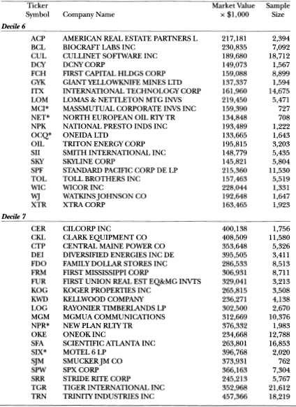
10.7 A Larger Sample

Although our sample of six securities contains several hundred thousand observations, it is still only a small cross-section of the ISSM database, which contains the transactions of over two thousand stocks. It would be impractical for us to estimate our ordered probit model for each one, so we apply our specification to a larger sample of 100 securities chosen randomly, twenty from each of market-value deciles 6 through 10 (decile 10 contains companies with beginning-of-year market values in the top 10% of the CRSP database), also with the restriction that none of these one hundred engaged in stock splits or stock dividends greater than or equal to 3:2. We also discarded (without replacement) randomly chosen stocks that were obviously mutual funds, replacing them with new random draws. Table 10.5 lists the companies' names, ticker symbols, market values, and number of trades included in our final samples.

Securities from deciles 1 through 5 were not selected because many of them are so thinly traded that the small sample sizes would not permit accurate estimation of the ordered probit parameters. For example, even in deciles 6, 7, and 8, containing companies ranging from $133 million to $946 million in market value, there were still six companies for which the maximum likelihood estimation procedure did not converge: MCI, NET, OCQ, NPR, SIX, and SW. In all of these cases, the sample sizes were relatively small, yielding ill-behaved and erratic likelihood functions.

Table 10.6. Summary statistics for the sample of 100 randomly chosen securities for the period from january 4, 1988, to December 30, 1988. Market values are computed at the beginning of the year.

¹ Five-minute continuouslycompounded returns of the S&P 500 index futures price, for the contract maturing in the closest month beyond the month in which transaction k occurred, where the return corresponding to the kth transaction of each stock is computed with the futures price recorded one minute before the nearest round minute prior to t_k and the price recorded five minutes before this.

² Takes the value 1 if the kth transaction price is greater than the average of the quoted bid and ask prices at time t_k, the value -1 if the kth transaction price is less than the average of the quoted bid and ask prices at time t_k, and 0 otherwise.

³ Box-Cox transformation of dollar volume multiplied by the buy/sell indicator, where the Box-Cox parameter λ is estimated jointly with the other ordered probit parameters via maximum likelihood.

⁴ Estimate of Box-Cox parameter λ which determines the degree of curvature that the transformation T_λ(•) exhibits in transforming dollar volume V_k before inclusion as an explanatory variable in the ordered probit specification. If λ = 1, the transformation T_λ(•) is linear, hence dollar volume enters the ordered probit model linearly. If λ = 0, the transformation is equivalent to log(•), hence the natural logarithm of dollar volume enters the ordered probit model. When λ is between 0 and 1, the curvature of T_x(•) is between logarithmic and linear.

 

Table 10.6 presents summary statistics for this sample of one hundred securities broken down by deciles. As expected, the larger stocks tend to have higher prices, shorter times between trades, higher bid/ask spreads (in ticks), and larger median dollar volume per trade. Note that the statistics for T_λ(V_k) • IBS_k implicidy include estimates of the Box-Cox parameter which differ across stocks. Also, although the mean and standard deviation of T_λ(V_k) • IBS_k for decile 6 differ dramatically from those of the other deciles, these differences are driven solely by the outlier XTR. When this security is dropped from decile 6, the mean and standard deviation of T_λ(V_k)IBS_k become -0.0244 and 0.3915, respectively, much more in line with the values of the other deciles.

In Table 10.7 we summarize the price impact measures across deciles, where we now define price impact to be the increase in the conditional expected price change as dollar volume increases from a base case of $1,000 to either the median dollar volume for each individual stock (the first panel of Table 10.7) or a dollar volume of $100,000 (the second panel). The first two rows of both panels report decile means and standard deviations of the absolute price impact (measured in ticks), whereas the second two rows of both panels report decile means and standard deviations of percentage price impact (measured as percentages of the mean of the high and low prices of each stock). For each stock i, we set ft and AB_k-i to their sample means for that stock and condition on the following values for the other regressors:

so that we are assuming the three most recent trades are buyer-initiated, accompanied by price increases of one tick each, and the sizes of the two earlier trades are equal to the median dollar volume of the particular stock in question.

From Table 10.7 we see that conditional on a dollar volume equal to the median for the most recent trade, larger capitalization stocks tend to exhibit larger absolute price impact, no doubt due to their higher prices and their larger median dollar volumes per trade. However, as percentages of the average of their high and low prices, the price impact across deciles is relatively constant as shown by the third row in the first panel of Table 10.7: the average price impact for a median trade in decile 6 is 0.0612%, compared to 0.0523% in decile 10. When conditioning on a dollar volume of $100,000, however, the results are quite different: the average absolute price impact is similar across deciles, but the average relative price impact is considerably smaller in decile 10 (0.0778%) than in decile 6 (0.2250%). Not surprisingly, a fixed $100,000 trade will have a greater percentage price impact on smaller capitalization, less liquid stocks than on larger ones.

Further insights on how price impact varies cross-sectionally can be gained from the cross-sectional regressions in Table 10.8, where the four price impact measures and the Box-Cox parameter estimates are each regressed on the following four variables: market value, the initial price level, median dollar volume, and median time-between-trades. Entries in the first row show that the Box-Cox parameters are inversely related to all four variables, though none of the coefficient estimates are statistically significant and the adjusted R² is negative, a symptom of the imprecision with which the λ_i's are estimated. But the two percentage price impact regressions seem to have higher explanatory power, with adjusted R²'s of 37.6% and 22.1%, respectively. These two regressions have identical sign patterns, implying that percentage price impact is larger for smaller stocks, lower-priced stocks, higher-volume stocks, and stocks that trade less frequently.

Table 10.7. Price impact measures, defined as the increase in conditional expected price change given by the ordered probit model as the volume of the most recent trade is increased from a base case of $1,000 to either the median level of volume for each security or a level of $100,000, for the sample of 100 randomly chosen securities for the period from january 4, 1988, to December 30, 1988. Price impact measures expressed in percent are percentages of the average of the high and low prices of each security.

 

Of course, these cross-sectional regressions are merely meant as data summaries, and may not correspond to well-specified regression equations. As a further check on the robustness of these regression-based inferences, in Table 10.9 we report Spearman rank correlations between the dependent and independent variables of Table 10.8, which are nonparametric measures of association and are asymptotically normal with mean 0 and variance 1/(n - 1) under the null hypothesis of pairwise independence (see,for example, Randles and Wolfe (1979)). Since n = 94, the twostandarderror confidence interval about zero for each of the correlation coefficients is [-0.207,0.207]. The sign patterns are much the same in Table 10.9 as in Table 10.8, despite the fact that the Spearman rank correlations are not partial correlation coefficients.

 

Table 10.8. Summary of the cross-sectional dispersion in price impact measures and the nonlinearity of the price-change/volume relation (as measured by the Box-Cox parameters, _i), via ordinary least-squares regressions for the sample of 100 randomly chosen securities, using market value, initial price, median volume, and median time-between-trades as explanatory variables, for the period from january 4, 1988, to December 30, 1988. Only 94 stocks are included in each of the regressions since the maximum likelihood estimation procedure did not converge for the omitted six. All the coefficents have been multiplied by afactor of 1,000, and z-statistics are given in parentheses, each of which is asymptotically distributed as (0, 1) under the null hypothesis that the corresponding coefficient is zero.

^lThe Box-Cox parameter λ, determines the degree of curvature that the transformation T_λ(•) exhibits in transforming dollar volume V_k before inclusion as an explanatory variable in the ordered probit specification. If λ = 1, the transformation T_λ(•) is linear, hence dollar volume enters the ordered probit model linearly. If λ = 0, the transformation is equivalent to log(•), hence the natural logarithm of dollar volume enters the ordered probit model. When λ is between 0 and 1, the curvature of T_λ(•) is between logarithmic and linear.

Such cross-sectional regressions and rank correlations serve only as informal summaries of the data since. They are not formally linked to any explicit theories of how price impact should vary across stocks. However, they are consistent with our earlier findings from the six stocks, suggesting that those results are not specific to the behavior of a few possibly peculiar stocks, but may be evidence of a more general and stable mechanism for transaction prices.

Table 10.9. Robust measure of the cross-sectional dispersion in price impact measures and the nonlinearity of the price-change/volume relation (as measured by the Box-Cox parameters _i), via the Spearman rank correlations of _i and price impact measures with market value, initial price, median volume, and median time-between-trades for the sample of 100 randomly chosen securities, of which 94 are used since the maximum likelihood estimation procedure did not converge for the omitted six, over the period from january 4, 1988, to December 30, 1988. Under the null hypothesis of independence, each of the correlation coefficients is asymptotically normal with mean 0 and variance l/( n–1), hence the two-standard-error confidence interval for these correlation coefficients is [-0.207, 0.207].

¹The Box-Cox parameter λ determines the degree of curvature that the transformation T_λ(•) exhibits in transforming dollar volume V_k before inclusion as an explanatory variable in the ordered probit specification. If λ = 1, the transformation is linear, hence dollar volume enters the ordered probit model linearly. If λ = 0, the transformation is equivalent to log(•), hence the natural logarithm of dollar volume enters the ordered probit model. When λ is between 0 and 1, the curvature of T_λ(•) is between logarithmic and linear.

10.8 Conclusion

Using 1988 transactions data from the ISSM database, we find that the sequence of trades does affect the conditional distribution for price changes, and the effect is greater for larger capitalization and more actively traded securities. Trade size is also an important factor in the conditional distribution of price changes, with larger trades creating more price pressure, but in a nonlinear fashion. The price impact of a trade depends critically on the sequence of past price changes and order flows (buy/sell/buy versus sell/buy/buy). The ordered probit framework allows us to compare the price impact of trading over many different market scenarios, such as trading “with” versus “against” the market, trading in “up” and “down” markets, etc. Finally, we show that discreteness does matter, in the sense that the simpler linear regression analysis of price changes cannot capture all the features of transaction price changes evident in the ordered probit estimates, such as the clustering of price changes on even eighths.

With these applications, we hope to have demonstrated the flexibility and power of the ordered probit model as a tool for investigating the dynamic behavior of transaction prices. Much like the linear regression model for continuous-valued data, the ordered probit model can capture and summarize complex relations between discrete-valued price changes and continuous-valued regressors. Indeed, even in the simple applications considered here, we suffer from an embarrassment of riches in that there are many other empirical implications of our ordered probit estimates that we do not have space to report. For example, we have compared the price impact of only one or two sequences of order flows, price history, and market returns, but there are many other combinations of market conditions, some that might yield considerably different findings. By selecting other scenarios, we may obtain a deeper and broader understanding of how transaction prices react to changing market conditions.

Although we have selected a wide range of regressors to illustrate the flexibility of ordered probit, in practice the specific application will dictate which regressors to include. If, for example, one is interested in testing the implications of Admati and Pfleiderer's (1988) model of intraday patterns in price and volume, natural regressors to include are time-ofday indicators in the conditional mean and variance. If one is interested in measuring how liquidity and price impact vary across markets, an exchange indicator would be appropriate. For intraday event studies, “event” indicators in both the conditional mean and variance are the natural regressors, and in such cases the generalized residuals we calculated as diagnostics can also be used to construct cumulative average (generalized) residuals.

In the few illustrative applications considered here, we have only hinted at the kinds of insights that ordered probit can yield. The possibilities increase exponentially as we consider the many ways our basic specification can be changed to accommodate the growing number of highly parametrized and less stylized theories about the market microstructure, and we expect to see many other applications in the near future.

---

¹see, for example, Glosten and Harris (1988), Hasbrouck (1988), Roll (1984a), and Stoll (1989).

²See Cohen et al. (1986), Harris, Sofianos, and Shapiro (1994), Hasbrouck (1991a, 1991b), Madhavan and Smidt (1991), and Stoll and Whaley (1990).

³The implications of discreteness have been considered in many studies, e.g., Cho and Frees (1988), Gottlieb and Kalay (1985), Harris (1989a, 1991), Petersen (1986), and Pritsker (1990).

⁴There is, however, a substantial literature on price/volume relations in which discreteness is ignored because of the return horizons involved (usually daily or longer). See, for example, Campbell, Grossman, and Wang (1991), Gallant, Rossi, and Tauchen (1992), and Karpoff (1987).

⁵The ordered probit model was developed by Aitchison and Silvey (1957) and Ashford (1959), and generalized to nonnormal disturbances by Gurland, Lee, and Dahm (1960). For more recent extensions, see Maddala (1983), McCullagh (1980), and Thisted (1991).

⁶Unless explicitly stated otherwise, all the probabilities we deal with in this study are conditional probabilities, and all statements concerning these probabilities are conditional statements, conditioned on these variables.

⁷ This rather convoluted timing for computing SP500_k-l ensures that there is no temporal overlap between price changes and the returns to the index futures price. In particular, we first construct a minute-by-minute time series for futures prices by assigning to each round minute the nearest futures transaction price occurring after that minute but before the next (hence if the first futures transaction after 10 : 35 : 00 occurs at 10 : 35 : 15, the futures price assigned to 10 : 35 : 00 is this one). If no transaction occurs during this minute, the price prevailing at the previous minute is assigned to the current minute. Then for the price change Z_k, we compute SP500_k-1 using the futures price one minute before the nearest round minute prior to t_k-1, and the price five minutes before this (hence if t_k-1 is 10 : 36 : 45, we use the futures price assigned to 10 : 35 : 00 and 10 : 30 : 00 to compute SP500_k-l).

⁸For example, the 99.5 percentile for IBM's share volume is 16,500 shares, hence all IBM trades exceeding 16,500 shares are set equal to 16,500 shares. By definition, only one-half of one percent of the 206,794 IBM trades (or 1,034 trades) were “censored” in this manner. We chose not to discard these trades because omitting them could affect our estimates of the lag structure, which is extremely sensitive to the sequence of trades. For the five remaining stocks, the 99.5 percentiles for share volume are: CUE = 21,300, FWC = 31,700, HNH = 20,000, NAV = 50,000, and T = 44,100.

⁹ In an earlier specification, in place of lagged price changes we included separate indicator variables for eight of the nine states of each lagged price change. But because the coefficients of the indicator variables increased monotonically from the -4 state to the +4 state (state 0 was omitted) in almost exact proportion to the tick change, we chose the more parsimonious specification of including the actual lagged price change.

¹⁰Just a few recent examples of this growing literature are Admati and Pfleiderer (1988), 1989), Amihud and Mendelson (1980), Easley and O'Hara (1987), Garman (1976), Glosten and Milgrom (1985), Grundy and McNichols (1989), Ho and Stoll (1980, 1981), Karpoff (1986), Kyle (1985), Stoll (1989), and Wang (1994).