Table 3-3 lists a variety of routines for matrix manipulation, most of which work equally well for images. They do all of the "usual" things, such as diagonalizing or transposing a matrix, as well as some more complicated operations, such as computing image statistics.
Table 3-3. Basic matrix and image operators
void cvAbs(
    const CvArr* src1,
    CvArr*        dst
);
void cvAbsDiff(
   const CvArr* src1,
   const CvArr* src2,
   CvArr*        dst
);
void cvAbsDiffS(
    const CvArr* src,
    CvArr*       dst,
    CvScalar     value,
);
These functions compute the absolute value of an array or of the difference between the array and some
reference. The cvAbs() function simply computes the
absolute value of the elements in src and writes the
result to dst; cvAbsDiff() first subtracts src2 from
src1 and then writes the absolute value of the
difference to dst. Note that cvAbsDiffS() is essentially the same as cvAbsDiff() except that the value subtracted from all of the elements of src is the
constant scalar value.
void cvAdd(
    const CvArr* src1,
    const CvArr* src2,
    CvArr*       dst,
    const CvArr* mask = NULL
);
void cvAddS(
    const CvArr* src,
    CvScalar     value,
    CvArr*       dst,
    const CvArr* mask = NULL
);
void cvAddWeighted(
    const CvArr* src1,
    double       alpha,
    const CvArr* src2,
    double       beta,
    double       gamma,
    CvArr*       dst
);
cvAdd() is a simple addition function: it adds
all of the elements in src1 to the corresponding
elements in src2 and puts the results in dst. If mask is not set
to NULL, then any element of dst that corresponds to a zero element of mask remains unaltered by this operation. The closely related function
cvAddS() does the same thing except that the
constant scalar value is added to every element of
src.
The function cvAddWeighted() is similar to
cvAdd() except that the result written to dst is computed according to the following formula:
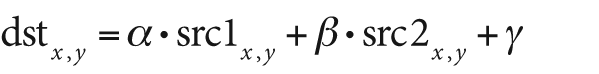
This function can be used to implement alpha blending [Smith79; Porter84]; that is, it can be used to blend one image with another. The form of this function is:
void  cvAddWeighted(
    const CvArr* src1,
    double       alpha,
    const CvArr* src2,
    double       beta,
    double       gamma,
    CvArr*       dst
);
In cvAddWeighted() we have two source images,
src1 and src2.
These images may be of any pixel type so long as both are of the same type. They may
also be one or three channels (grayscale or color), again as long as they agree. The
destination result image, dst, must also have the
same pixel type as src1 and src2. These images may be of different sizes, but their ROIs must agree in
size or else OpenCV will issue an error. The parameter alpha is the blending strength of src1,
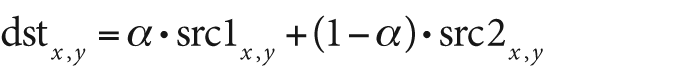
and beta is the blending strength of src2. The alpha blending equation is:

You can convert to the standard alpha blend equation by choosing α between 0 and 1, setting β = 1 − α, and setting γ to 0; this yields:
However, cvAddWeighted() gives us a little more
flexibility—both in how we weight the blended images and in the additional parameter γ,
which allows for an additive offset to the resulting destination image. For the general
form, you will probably want to keep alpha and
beta at no less than 0 and their sum at no more
than 1; gamma may be set depending on average or max
image value to scale the pixels up. A program showing the use of alpha blending is shown
in Example 3-14.
Example 3-14. Complete program to alpha blend the ROI starting at (0,0) in src2 with the ROI starting at (x,y) in src1
// alphablend <imageA> <image B> <x> <y> <width> <height>
// <alpha> <beta>
#include <cv.h>
#include <highgui.h>
int main(int argc, char** argv)
{
IplImage *src1, *src2;
if( argc == 9 && ((src1=cvLoadImage(argv[1],1)) != 0
)&&((src2=cvLoadImage(argv[2],1)) != 0 ))
{
int x = atoi(argv[3]);
int y = atoi(argv[4]);
int width = atoi(argv[5]);
int height = atoi(argv[6]);
double alpha = (double)atof(argv[7]);
double beta = (double)atof(argv[8]);
cvSetImage ROI(src1, cvRect(x,y,width,height));
cvSetImageROI(src2, cvRect(0,0,width,height));
cvAddWeighted(src1, alpha, src2, beta,0.0,src1);
cvResetImageROI(src1);
cvNamedWindow( "Alpha_blend", 1 );
cvShowImage( "Alpha_blend", src1 );
cvWaitKey();
}
return 0;
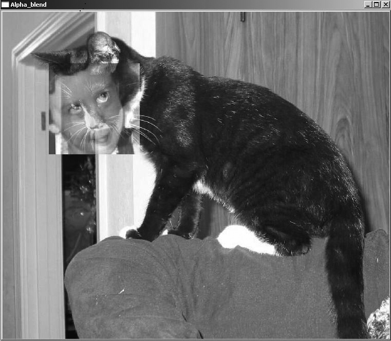
}The code in Example 3-14 takes two
source images: the primary one (src1) and the one to
blend (src2). It reads in a rectangle ROI for
src1 and applies an ROI of the same size to
src2, this time located at the origin. It reads in
alpha and beta
levels but sets gamma to 0.Alpha blending is applied using cvAddWeighted(), and the results are put into src1 and displayed. Example output is shown in Figure 3-4, where the face of a child is
blended onto the face and body of a cat. Note that the code took the same ROI as in the
ROI addition example in Figure 3-3. This
time we used the ROI as the target blending region.
void cvAnd(
    const CvArr* src1,
    const CvArr* src2,
    CvArr*       dst,
    const CvArr* mask = NULL
);
void cvAndS(
    const CvArr* src1,
    CvScalar     value,
    CvArr*       dst,
    const CvArr* mask = NULL
);
These two functions compute a bitwise AND operation on the array src1.
In the case of cvAnd(), each element of dst is computed as the bitwise AND of the corresponding two
elements of src1 and src2. In the case of cvAndS(), the
bitwise AND is computed with the constant scalar value. As always, if mask is
non-NULL then only the elements of dst corresponding to nonzero entries in mask are computed.
Though all data types are supported, src1 and
src2 must have the same data type for cvAnd(). If the elements are of a floating-point type, then
the bitwise representation of that floating-point number is used.
CvScalar cvAvg(
    const CvArr* arr,
    const CvArr* mask = NULL
);
cvAvg() computes the average value of the pixels
in arr. If mask is
non-NULL then the average will be computed only
over those pixels for which the corresponding value of mask is nonzero.
cvAvgSdv(
    const CvArr* arr,
    CvScalar*    mean,
    CvScalar*    std_dev,
    const CvArr* mask     = NULL
);
This function is like cvAvg(), but in addition to
the average it also computes the standard deviation of the pixels.
void cvCalcCovarMatrix(
    const CvArr** vects,
    int           count,
    CvArr*        cov_mat,
    CvArr*        avg,
    int           flags
);
Given any number of vectors, cvCalcCovarMatrix()
will compute the mean and covariance matrix for the Gaussian
approximation to the distribution of those points. This can be used in many ways, of
course, and OpenCV has some additional flags that will help in particular contexts (see
Table 3-4). These flags may be
combined by the standard use of the Boolean OR operator.
In all cases, the vectors are supplied in vects
as an array of OpenCV arrays (i.e., a pointer to a list of pointers to arrays), with the argument
count indicating how many arrays are being
supplied. The results will be placed in cov_mat in
all cases, but the exact meaning of avg depends on
the flag values (see Table 3-4).
The flags CV_COVAR_NORMAL and CV_COVAR_SCRAMBLED are mutually exclusive; you should use
one or the other but not both. In the case of CV_COVAR_NORMAL, the function will simply compute the mean and covariance
of the points provided.
Thus the normal covariance  is computed from the m vectors of length
n, where
is computed from the m vectors of length
n, where  is defined as the nth element of the average
vector
is defined as the nth element of the average
vector  . The resulting covariance matrix is an
n-by-n matrix. The factor
z is an optional scale factor; it will be set to 1 unless the
. The resulting covariance matrix is an
n-by-n matrix. The factor
z is an optional scale factor; it will be set to 1 unless the
CV_COVAR_SCALE flag is used.
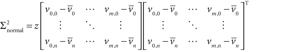
In the case of CV_COVAR_SCRAMBLED,
cvCalcCovarMatrix() will compute the following:
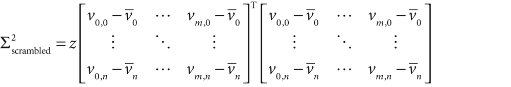
This matrix is not the usual covariance matrix (note the location of the transpose operator). This matrix is computed from the same m vectors of length n, but the resulting scrambled covariance matrix is an m-by-m matrix. This matrix is used in some specific algorithms such as fast PCA for very large vectors (as in the eigenfaces technique for face recognition).
The flag CV_COVAR_USE_AVG is used when the mean
of the input vectors is already known. In this case, the argument avg is used as an input rather than an output, which reduces
computation time.
Finally, the flag CV_COVAR_SCALE is used to apply
a uniform scale to the covariance matrix calculated. This is the factor
z in the preceding equations. When used in conjunction with the
CV_COVAR_NORMAL flag, the applied scale factor will
be 1.0/m (or, equivalently,
1.0/count). If instead CV_COVAR_SCRAMBLED is used, then the value of z will
be 1.0/n (the inverse of the
length of the vectors).
The input and output arrays to cvCalcCovarMatrix() should all be of the same floating-point type. The size
of the resulting matrix cov_mat should be either
n-by-n or
m-by-m depending on whether the standard or
scrambled covariance is being computed. It should be noted that the "vectors" input in
vects do not actually have to be one-dimensional;
they can be two-dimensional objects (e.g., images) as well.
void cvCmp(
    const CvArr* src1,
    const CvArr* src2,
    CvArr*       dst,
    int          cmp_op
);
void cvCmpS(
    const CvArr* src,
    double       value,
    CvArr*       dst,
    int          cmp_op
);
Both of these functions make comparisons, either between corresponding pixels in two
images or between pixels in one image and a constant scalar value. Both cvCmp() and cvCmpS() take
as their last argument a comparison operator, which may be any of the types listed in
Table 3-5.
Table 3-5. Values of cmp_op used by cvCmp() and cvCmpS() and the resulting comparison operation performed
|
Value of cmp_op |
Comparison |
|---|---|
|
|
|
|
|
|
|
|
|
|
|
|
|
|
|
|
|
|
All the listed comparisons are done with the same functions; you just pass in the appropriate argument to indicate what you would like done. These particular functions operate only on single-channel images.
These comparison functions are useful in applications where you employ some version of background subtraction and want to mask the results (e.g., looking at a video stream from a security camera) such that only novel information is pulled out of the image.
The cvConvertScale() function is actually several
functions rolled into one; it will perform any of several functions or, if desired, all
of them together. The first function is to convert the data type in the source image to the data type of the destination image. For
example, if we have an 8-bit RGB grayscale image and would like to convert it to a
16-bit signed image, we can do that by calling cvConvertScale().
The second function of cvConvertScale() is to
perform a linear transformation on the image data. Each pixel value will be multiplied
by the value scale and then have added to it the
value shift. It is critical to remember that, even
though "Convert" precedes "Scale" in the function name, the actual order in which these
operations is performed is the opposite (i.e. multiplication by scale and the addition of shift occurs
before the type conversion takes place).
When you simply pass the default values (scale =
1.0 and shift = 0.0), you need not have
performance fears; OpenCV is smart enough to recognize this case and not waste processor
time on useless operations. For clarity (if you think it adds any), OpenCV also provides
the macro cvConvert(), which is the same as cvConvertScale() but is conventionally used when the
scale and shift
arguments will be left at their default values.
cvConvertScale() will work on all data types and
any number of channels, but the number of channels in the source and destination images
must be the same. (If you want to, say, convert from color to grayscale or vice versa,
see cvCvtColor(), which is coming up shortly.)
void cvConvertScaleAbs(
    const CvArr* src,
    CvArr*       dst,
    double       scale = 1.0,
    double       shift = 0.0
);
cvConvertScaleAbs() is essentially identical to
cvConvertScale() except that the dst image contains the absolute value of the resulting data. Specifically, cvConvertScaleAbs() first scales and shifts, then computes the absolute
value, and finally performs the data-type conversion.
void cvCopy(
    const CvArr* src,
    CvArr*       dst,
    const CvArr* mask = NULL
);
This is how you copy one image to another. The cvCopy() function expects both arrays to have the same type, the same size,
and the same number of dimensions. You can use it to copy sparse arrays as well, but for
this the use of mask is not supported. For nonsparse
arrays and images, the effect of mask (if
non-NULL) is that only the pixels in dst that correspond to nonzero entries in mask will be altered.
int cvCountNonZero( const CvArr* arr );
cvCountNonZero() returns the number of nonzero
pixels in the array arr.
void cvCrossProduct(
    const CvArr* src1,
    const CvArr* src2,
    CvArr*       dst
);
This function computes the vector cross product [Lagrange1773] of two
three-dimensional vectors. It does not matter if the vectors are in row or column form
(a little reflection reveals that, for single-channel objects, these two are really the
same internally). Both src1 and src2 should be single-channel arrays, and dst should be single-channel and of length exactly 3.All
three arrays should be of the same data type.
void cvCvtColor(
    const CvArr* src,
    CvArr*       dst,
    int          code
);
The previous functions were for converting from one data type to another, and they
expected the number of channels to be the same in both source and destination images.
The complementary function is cvCvtColor(), which
converts from one color space (number of channels) to another [Wharton71] while expecting the
data type to be the same. The exact conversion operation to be done is specified by the
argument code, whose possible values are listed in
Table 3-6.[25]
Table 3-6. Conversions available by means of cvCvtColor()
The details of many of these conversions are nontrivial, and we will not go into the subtleties of Bayer representations and the CIE color spaces here. For our purposes, it is sufficient to note that OpenCV contains tools to convert to and from these various color spaces, which are of importance to various classes of users.
The color-space conversions all use the conventions: 8-bit images are in the range 0–255, 16-bit images are in the range 0–65536, and floating-point numbers are in the range 0.0–1.0. When grayscale images are converted to color images, all components of the resulting image are taken to be equal; but for the reverse transformation (e.g., RGB or BGR to grayscale), the gray value is computed using the perceptually weighted formula:

In the case of HSV or HLS representations, hue is normally represented as a value from 0 to 360.[26] This can cause trouble in 8-bit representations and so, when converting to HSV, the hue is divided by 2 when the output image is an 8-bit image.
double cvDet(
    const CvArr* mat
);
cvDet() computes the determinant (Det) of a
square array. The array can be of any data type, but it must be
single-channel. If the matrix is small then the determinant is directly computed by the
standard formula. For large matrices, this is not particularly efficient and so the
determinant is computed by Gaussian elimination.
It is worth noting that if you already know that a matrix is symmetric and has a
positive determinant, you can also use the trick of solving via singular value
decomposition (SVD). For more information see the section "cvSVD" to follow, but the trick
is to set both U and V to
NULL and then just take the products of the matrix
W to obtain the determinant.
void cvDiv(
    const CvArr* src1,
    const CvArr* src2,
    CvArr*       dst,
    double       scale = 1
);
cvDiv() is a simple division function; it divides
all of the elements in src1 by the corresponding
elements in src2 and puts the results in dst. If mask is
non-NULL, then any element of dst that corresponds to a zero element of mask is not altered by this operation. If you only want to
invert all the elements in an array, you can pass NULL in the place of src1; the routine
will treat this as an array full of 1s.
double cvDotProduct(
    const CvArr* src1,
    const CvArr* src2
);
This function computes the vector dot product [Lagrange1773] of two
N-dimensional vectors.[27] As with the cross product (and for the same reason), it does not matter if
the vectors are in row or column form. Both src1 and
src2 should be single-channel arrays, and both
arrays should be of the same data type.
double cvEigenVV(
    CvArr* mat,
    CvArr* evects,
    CvArr* evals,
    double eps    = 0
);
Given a symmetric matrix mat, cvEigenVV() will
compute the eigenvectors and the corresponding
eigenvalues of that matrix. This is done using Jacobi's
method [Bronshtein97], so it is efficient for smaller matrices.[28] Jacobi's method requires a stopping parameter, which is the maximum size of
the off-diagonal elements in the final matrix.[29] The optional argument eps sets this
termination value. In the process of computation, the supplied matrix mat is used for the computation, so its values will be
altered by the function. When the function returns, you will find your eigenvectors in
evects in the form of subsequent rows. The
corresponding eigenvalues are stored in evals. The
order of the eigenvectors will always be in descending order of the magnitudes of the
corresponding eigenvalues. The cvEigenVV() function
requires all three arrays to be of floating-point type.
As with cvDet() (described previously), if the
matrix in question is known to be symmetric and positive definite[30] then it is better to use SVD to find the eigenvalues and eigenvectors of mat.
void cvFlip(
    const CvArr* src,
    CvArr*       dst       = NULL,
    int          flip_mode = 0
);
This function flips an image around the x-axis, the
y-axis, or both. In particular, if the argument flip_mode is set to 0 then the image will be flipped around
the x-axis.
If flip_mode is set to a positive value (e.g.,
+1) the image will be flipped around the
y-axis, and if set to a negative value (e.g., –1) the image will be flipped about both axes.
When video processing on Win32 systems, you will find yourself using this function often to switch between image formats with their origins at the upper-left and lower-left of the image.
double cvGEMM(
    const CvArr* src1,
    const CvArr* src2,
    double       alpha,
    const CvArr* src3,
    double       beta,
    CvArr*       dst,
    int          tABC = 0
);
Generalized matrix multiplication (GEMM) in OpenCV is performed by cvGEMM(), which performs matrix multiplication, multiplication by a transpose, scaled multiplication, et
cetera. In its most general form, cvGEMM() computes
the following:
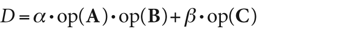
Where A, B, and C are
(respectively) the matrices src1, src2, and src3, α and β are
numerical coefficients, and op() is an optional transposition of the matrix enclosed.
The argument src3 may be set to NULL, in which case it will not be added. The transpositions
are controlled by the optional argument tABC, which
may be 0 or any combination (by means of Boolean OR) of CV_GEMM_A_T, CV_GEMM_B_T, and CV_GEMM_C_T (with each flag indicating a transposition of the corresponding
matrix).
In the distant past OpenCV contained the methods cvMatMul() and cvMatMulAdd(), but these
were too often confused with cvMul(), which does
something entirely different (i.e., element-by-element multiplication of two arrays).
These functions continue to exist as macros for calls to cvGEMM(). In particular, we have the equivalences listed in Table 3-7.
Table 3-7. Macro aliases for common usages of cvGEMM()
|
|
|
|
|
|
All matrices must be of the appropriate size for the multiplication, and all should
be of floating-point type. The cvGEMM() function
supports two-channel matrices, in which case it will treat the two channels as the two
components of a single complex number.
CvMat* cvGetCol(
    const CvArr* arr,
    CvMat*       submat,
    int          col
);
CvMat* cvGetCols(
    const CvArr* arr,
    CvMat*       submat,
    int          start_col,
    int          end_col
);
The function cvGetCol() is used to pick a single
column out of a matrix and return it as a vector (i.e., as a matrix with only one
column). In this case the matrix header submat will
be modified to point to a particular column in arr.
It is important to note that such header modification does not include the allocation of
memory or the copying of data. The contents of submat
will simply be altered so that it correctly indicates the selected column in arr. All data types are supported.
cvGetCols() works precisely the same way, except
that all columns from start_col to end_col are selected. With both functions, the return value
is a pointer to a header corresponding to the particular specified column or column span
(i.e., submat) selected by the caller.
CvMat* cvGetDiag(
    const CvArr* arr,
    CvMat*       submat,
    int          diag    = 0
);
cvGetDiag() is analogous to cvGetCol(); it is used to pick a single
diagonal from a matrix and return it as a vector. The argument
submat is a matrix header. The function cvGetDiag() will fill the components of this header so that
it points to the correct information in arr. Note
that the result of calling cvGetDiag() is that the
header you supplied is correctly configured to point at the diagonal data in arr, but the data from arr is not copied. The optional argument diag specifies which diagonal is to be pointed to by submat. If diag is set to
the default value of 0, the main diagonal will be selected. If diag is greater than 0, then the diagonal starting at (diag,0) will be selected; if diag is less than 0, then the diagonal starting at (0,-diag) will be selected instead. The cvGetDiag() function does not require the matrix arr to be square, but the array submat
must have the correct length for the size of the input array. The final returned value
is the same as the value of submat passed in when the
function was called.
int cvGetDims(
    const CvArr* arr,
    int*         sizes=NULL
);
int cvGetDimSize(
    const CvArr* arr,
    int          index
);
Recall that arrays in OpenCV can be of dimension much greater than two. The function
cvGetDims() returns the number of array dimensions
of a particular array and (optionally) the sizes of each of those dimensions. The sizes
will be reported if the array sizes is non-NULL. If sizes is used,
it should be a pointer to n integers, where n
is the number of dimensions. If you do not know the number of dimensions in advance, you
can allocate sizes to CV_MAX_DIM integers just to be safe.
If the array passed to cvGetDims() is either a matrix or an
image, the number of dimensions returned will always be two.[31] For matrices and images, the order of sizes returned by cvGetDims() will
always be the number of rows first followed by the number of columns. The function
cvGetDimSize() returns the size of a single
dimension specified by index.
CvMat* cvGetRow(
    const CvArr* arr,
    CvMat*       submat,
    int          row
);
CvMat* cvGetRows(
    const CvArr* arr,
    CvMat*       submat,
    int          start_row,
    int          end_row
);
cvGetRow() picks a single row out of a matrix and
returns it as a vector (a matrix with only one row). As with cvGetCol(), the matrix header submat
will be modified to point to a particular row in arr,
and the modification of this header does not include the allocation of memory or the
copying of data; the contents of submat will simply
be altered such that it correctly indicates the selected row in arr. All data types are supported.
The function cvGetRows() works precisely the same
way, except that all rows from start_row to end_row are selected. With both functions, the return value
is a pointer to a header corresponding to the particular specified row or row span
selected by the caller.
CvSize cvGetSize( const CvArr* arr );
Closely related to cvGetDims(), cvGetSize()
returns the size of an array. The primary difference is that cvGetSize() is designed to be used on matrices and images, which always
have dimension two. The size can then be returned in the form of a CvSize structure, which is suitable to use when (for
example) constructing a new matrix or image of the same size.
CvMat* cvGetSubRect(
    const CvArr* arr,
    CvMat*       submat,
    CvRect       rect
);
cvGetSubRect() is similar to cvGetCols() or cvGetRows() except that it selects some arbitrary subrectangle in the array
specified by the argument rect. As with other
routines that select subsections of arrays, submat is
simply a header that will be filled by cvGetSubRect()
in such a way that it correctly points to the desired submatrix (i.e., no memory is
allocated and no data is copied).
void cvInRange(
    const CvArr* src,
    const CvArr* lower,
    const CvArr* upper,
    CvArr*       dst
);
void cvInRangeS(
    const CvArr* src,
    CvScalar     lower,
    CvScalar     upper,
    CvArr*       dst
);
These two functions can be used to check if the pixels in an image fall within a
particular specified range. In the case of cvInRange(), each pixel of src is
compared with the corresponding value in the images lower and upper. If the value in
src is greater than or equal to the value in
lower and also less than the value in upper, then the corresponding value in dst will be set to 0xff;
otherwise, the value in dst will be set to
0.
The function cvInRangeS() works precisely the
same way except that the image src is compared to the
constant (CvScalar) values in lower and upper. For both
functions, the image src may be of any type; if it
has multiple channels then each channel will be handled separately. Note that dst must be of the same size and number of channels and also
must be an 8-bit image.
double cvInvert(
    const CvArr* src,
    CvArr*       dst,
    int          method = CV_LU
);
cvInvert() inverts the matrix in src and places the result in dst. This function supports several methods of computing the inverse matrix
(see Table 3-8), but the default is
Gaussian elimination. The return value depends on the method used.
In the case of Gaussian elimination (method=CV_LU), the determinant of src is
returned when the function is complete. If the determinant is 0, then the inversion is
not actually performed and the array dst is simply
set to all 0s.
In the case of CV_SVD or CV_SVD_SYM, the return value is the inverse condition number for the matrix
(the ratio of the smallest to the largest eigenvalue). If the matrix src is singular, then cvInvert() in SVD mode will instead compute the pseudo-inverse.
CvSize cvMahalanobis(
    const CvArr* vec1,
    const CvArr* vec2,
    CvArr*       mat
);
The Mahalanobis distance is defined as the vector distance measured between a point and the center of a Gaussian distribution; it is computed using the inverse covariance of that distribution as a metric. See Figure 3-5. Intuitively, this is analogous to the z-score in basic statistics, where the distance from the center of a distribution is measured in units of the variance of that distribution. The Mahalanobis distance is just a multivariable generalization of the same idea.
cvMahalanobis() computes the value:
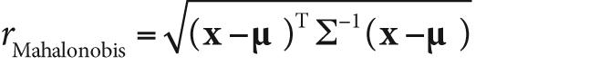
The vector vec1 is presumed to be the point
x, and the vector vec2 is taken to be the distribution's mean.[32] That matrix mat is the inverse
covariance.
In practice, this covariance matrix will usually have been computed with cvCalcCovarMatrix() (described previously) and then inverted
with cvInvert(). It is good programming practice to
use the SV_SVD method for this inversion because
someday you will encounter a distribution for which one of the eigenvalues is 0!
void cvMax(
    const CvArr* src1,
    const CvArr* src2,
    CvArr*       dst
);
void cvMaxS(
    const CvArr* src,
    double       value,
    CvArr*       dst
);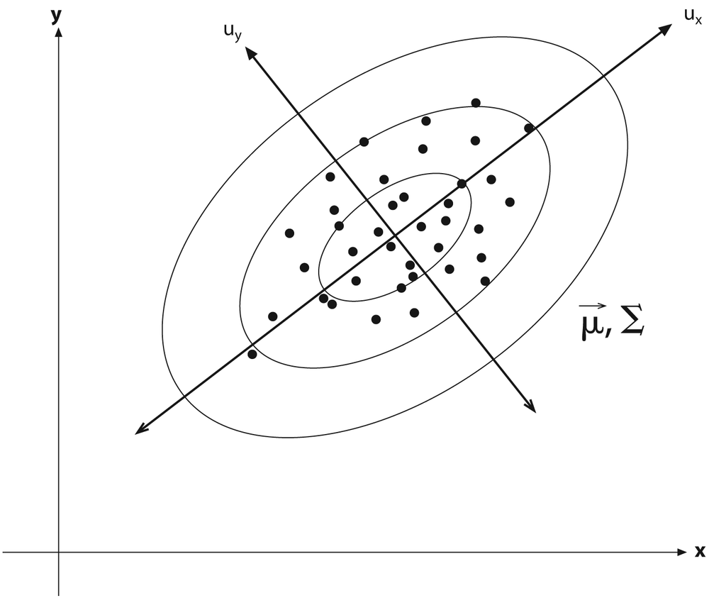
Figure 3-5. A distribution of points in two dimensions with superimposed ellipsoids representing Mahalonobis distances of 1.0, 2.0, and 3.0 from the distribution's mean
cvMax() computes the maximum value of each
corresponding pair of pixels in the arrays src1 and
src2. With cvMaxS(), the src array is compared with
the constant scalar value. As always, if mask is non-NULL then
only the elements of dst corresponding to nonzero
entries in mask are computed.
void cvMerge(
    const CvArr* src0,
    const CvArr* src1,
    const CvArr* src2,
    const CvArr* src3,
    CvArr* dst
);
cvMerge() is the inverse operation of cvSplit(). The arrays in src0,
src1, src2, and src3 are combined into
the array dst. Of course, dst should have the same data type and size as all of the source arrays,
but it can have two, three, or four channels. The unused source images can be left set
to NULL.
void cvMin(
    const CvArr* src1,
    const CvArr* src2,
    CvArr* dst
);
void cvMinS(
    const CvArr* src,
    double value,
    CvArr* dst
);
cvMin() computes the minimum value of each
corresponding pair of pixels in the arrays src1 and
src2. With cvMinS(), the src arrays are compared
with the constant scalar value. Again, if mask is non-NULL then
only the elements of dst corresponding to nonzero
entries in mask are computed.
void cvMinMaxLoc(
    const CvArr* arr,
    double*      min_val,
    double*      max_val,
    CvPoint*     min_loc = NULL,
    CvPoint*     max_loc = NULL,
    const CvArr* mask    = NULL
);
This routine finds the minimal and maximal values in the array arr and (optionally) returns their locations. The computed
minimum and maximum values are placed in min_val and
max_val. Optionally, the locations of those extrema
will also be written to the addresses given by min_loc and max_loc if those values are
non-NULL.
As usual, if mask is non-NULL then only those portions of the image arr that correspond to nonzero pixels in mask are considered. The cvMinMaxLoc()
routine handles only single-channel arrays, however, so if you have a multichannel array
then you should use cvSetCOI() to set a particular
channel for consideration.
void cvMul(
    const CvArr* src1,
    const CvArr* src2,
    CvArr* dst,
    double scale=1
);
cvMul() is a simple multiplication function. It multiplies all of the elements in src1 by the corresponding elements in src2 and then puts the results in dst. If mask is non-NULL, then any element of dst that corresponds to a zero element of mask is not altered by this operation. There is no function cvMulS() because that functionality is already provided by
cvScale() or cvConvertScale().
One further thing to keep in mind: cvMul()
performs element-by-element multiplication. Someday, when you are multiplying some
matrices, you may be tempted to reach for cvMul().
This will not work; remember that matrix multiplication is done with cvGEMM(), not cvMul().
cvNot(
    const CvArr* src,
    CvArr*       dst
);
The function cvNot() inverts every bit in every
element of src and then places the result in dst. Thus, for an 8-bit image the value 0x00 would be mapped
to 0xff and the value 0x83 would be mapped to 0x7c.
double cvNorm(
    const CvArr* arr1,
    const CvArr* arr2      = NULL,
    int          norm_type = CV_L2,
    const CvArr* mask      = NULL
);
This function can be used to compute the total norm of an array and also a variety of relative distance norms if two arrays are provided. In the former case, the norm computed is shown in Table 3-9.

If the second array argument arr2 is non-NULL, then the norm computed is a difference norm—that is,
something like the distance between the two arrays.[33] In the first three cases shown in Table 3-10, the norm is absolute; in the
latter three cases it is rescaled by the magnitude of the second array arr2.


In all cases, arr1 and arr2 must have the same size and number of channels. When there is more
than one channel, the norm is computed over all of the channels together (i.e., the sums
in Tables Table 3-9 and Table 3-10 are not only over
x and y but also over the
channels).
cvNormalize(
    const CvArr* src,
    CvArr*       dst,
    double       a         = 1.0,
    double       b         = 0.0,
    int          norm_type = CV_L2,
    const CvArr* mask      = NULL
);
As with so many OpenCV functions, cvNormalize()
does more than it might at first appear. Depending on the value of norm_type, image src is
normalized or otherwise mapped into a particular range in dst. The possible values of norm_type
are shown in Table 3-11.


In the case of the C norm, the array src is
rescaled such that the magnitude of the absolute value of the largest entry is equal to
a. In the case of the L1 or L2 norm, the array is
rescaled so that the given norm is equal to the value of a. If norm_type is set to CV_MINMAX, then the values of the array are rescaled and
translated so that they are linearly mapped into the interval between a and b
(inclusive).
As before, if mask is non-NULL then only those pixels corresponding to nonzero values
of the mask image will contribute to the computation of the norm—and only those pixels
will be altered by cvNormalize().
void cvOr(
    const CvArr* src1,
    const CvArr* src2,
    CvArr*       dst,
    const CvArr* mask=NULL
);
void cvOrS(
    const CvArr* src,
    CvScalar     value,
    CvArr*       dst,
    const CvArr* mask  = NULL
);
These two functions compute a bitwise OR operation on the array src1.
In the case of cvOr(), each element of dst is computed as the bitwise OR of the corresponding two
elements of src1 and src2. In the case of cvOrS(), the
bitwise OR is computed with the constant scalar value. As usual, if mask is non-NULL then only the elements of dst corresponding to nonzero entries in mask are computed.
All data types are supported, but src1 and
src2 must have the same data type for cvOr(). If the elements are of floating-point type, then the
bitwise representation of that floating-point number is used.
CvSize cvReduce(
    const CvArr* src,
    CvArr*       dst,
    int          dim,
    int          op = CV_REDUCE_SUM
);
Reduction is the systematic transformation of the input matrix src into a vector dst by
applying some combination rule op on each row (or
column) and its neighbor until only one row (or column) remains (see Table 3-12).[34] The argument dim controls how the
reduction is done, as summarized in Table 3-13.
Table 3-12. Argument op in cvReduce() selects the reduction operator
|
Value of op |
Result |
|---|---|
|
|
Compute sum across vectors |
|
|
Compute average across vectors |
|
|
Compute maximum across vectors |
|
|
Compute minimum across vectors |
Table 3-13. Argument dim in cvReduce() controls the direction of the reduction
|
Value of dim |
Result |
|---|---|
|
|
Collapse to a single row |
|
|
Collapse to a single column |
|
|
Collapse as appropriate for |
cvReduce() supports multichannel arrays of
floating-point type. It is also allowable to use a higher precision type in dst than appears in src.
This is primarily relevant for CV_REDUCE_SUM and
CV_REDUCE_AVG, where overflows and summation
problems are possible.
void cvRepeat(
    const CvArr* src,
    CvArr*       dst
);
This function copies the contents of src into
dst, repeating as many times as necessary to fill
dst. In particular, dst can be of any size relative to src.
It may be larger or smaller, and it need not have an integer relationship between any of
its dimensions and the corresponding dimensions of src.
void cvScale(
    const CvArr* src,
    CvArr*       dst,
    double       scale
);
The function cvScale() is actually a macro for
cvConvertScale() that sets the shift argument to 0.0.
Thus, it can be used to rescale the contents of an array and to convert from one kind of
data type to another.
void cvSet(
    CvArr*       arr,
    CvScalar     value,
    const CvArr* mask   = NULL
);
These functions set all values in all channels of the array to a specified value. The cvSet()
function accepts an optional mask argument: if a mask
is provided, then only those pixels in the image arr
that correspond to nonzero values of the mask image
will be set to the specified value. The function
cvSetZero() is just a synonym for cvSet(0.0).
void cvSetIdentity( CvArr* arr );
cvSetIdentity() sets all elements of the array to 0 except for elements whose row and column are
equal; those elements are set to 1. cvSetIdentity()
supports all data types and does not even require the array to be square.
int cvSolve(
    const CvArr* src1,
    const CvArr* src2,
    CvArr*       dst,
    int          method = CV_LU
);
The function cvSolve() provides a fast way to
solve linear systems based on cvInvert(). It computes
the solution to
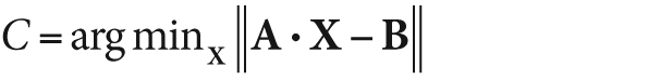
where A is a square matrix given by src1, B is the vector
src2, and C is the solution
computed by cvSolve() for the best vector X it could find. That best vector X is returned in dst. The same methods
are supported as by cvInvert() (described
previously); only floating-point data types are supported. The function returns an
integer value where a nonzero return indicates that it could find a solution.
It should be noted that cvSolve() can be used to
solve overdetermined linear systems. Overdetermined systems will be solved using
something called the pseudo-inverse, which uses SVD methods to find
the least-squares solution for the system of equations.
void cvSplit(
    const CvArr* src,
    CvArr*       dst0,
    CvArr*       dst1,
    CvArr*       dst2,
    CvArr*       dst3
);
There are times when it is not convenient to work with a multichannel image. In such
cases, we can use cvSplit() to copy each channel
separately into one of several supplied single-channel images. The cvSplit() function will copy the channels in src into the images dst0, dst1,
dst2, and dst3 as needed. The destination
images must match the source image in size and data type but, of course, should be
single-channel images.
If the source image has fewer than four channels (as it often will), then the
unneeded destination arguments to cvSplit() can be
set to NULL.
void cvSub(
    const CvArr* src1,
    const CvArr* src2,
    CvArr*       dst,
    const CvArr* mask  = NULL
);
void cvSubS(
    const CvArr* src,
    CvScalar     value,
    CvArr*       dst,
    const CvArr* mask  = NULL
);
void cvSubRS(
    const CvArr* src,
    CvScalar     value,
    CvArr*       dst,
    const CvArr* mask  = NULL
);
The closely related function cvSubS() does the
same thing except that the constant scalar value is
suntracted to every element of src. The function
cvSubRS() is the same as cvSubS() except that, rather than subtracting a constant from every element
of src, it subtracts every element of src from the constant value.
CvScalar cvSum(
    CvArr* arr
);
cvSum() sums all of the pixels in all of the
channels of the array arr. Observe that the return
value is of type CvScalar, which means that cvSum() can accommodate multichannel arrays. In that case,
the sum for each channel is placed in the corresponding component of the CvScalar return value.
void cvSVD(
    CvArr* A,
    CvArr* W,
    CvArr* U     = NULL,
    CvArr* V     = NULL,
    int    flags = 0
);
Singular value decomposition (SVD) is the decomposing of an m-by-n matrix A into the form:

where W is a diagonal matrix and U and V are m-by-m and n-by-n unitary matrices. Of course the matrix W is also an m-by-n matrix, so here "diagonal" means that any element whose row and column numbers are not equal is necessarily 0. Because W is necessarily diagonal, OpenCV allows it to be represented either by an m-by-n matrix or by an n-by-1 vector (in which case that vector will contain only the diagonal "singular" values).
The matrices U and V are optional to cvSVD(), and if they
are left set to NULL then no value will be returned.
The final argument flags can be any or all of the three options described in Table 3-14 (combined as appropriate with the
Boolean OR operator).
void cvSVBkSb(
    const CvArr* W,
    const CvArr* U,
    const CvArr* V,
    const CvArr* B,
    CvArr* X,
    int    flags = 0
);
This is a function that you are unlikely to call directly. In conjunction with
cvSVD() (just described), it underlies the
SVD-based methods of cvInvert() and cvSolve(). That being said, you may want to cut out the
middleman and do your own matrix inversions (depending on the data source, this could
save you from making a bunch of memory allocations for temporary matrices inside of
cvInvert() or cvSolve()).
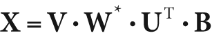
The function cvSVBkSb() computes the
back-substitution for a matrix A that is represented in
the form of a decomposition of matrices U, W, and V (e.g., an SVD). The result matrix X is given by the formula:
The matrix B is optional, and if set to NULL it will be ignored. The matrix W* is a matrix whose diagonal elements are defined by
for  . This value ε is the singularity threshold, a very small number that is
typically proportional to the sum of the diagonal elements of W (i.e.,
. This value ε is the singularity threshold, a very small number that is
typically proportional to the sum of the diagonal elements of W (i.e.,
CvScalar cvTrace( const CvArr* mat );
The trace of a matrix (Trace) is the sum of all of the diagonal elements. The trace
in OpenCV is implemented on top of the cvGetDiag()
function, so it does not require the array passed in to be square. Multichannel arrays
are supported, but the array mat should be of
floating-point type.
void cvTranspose(
    const CvArr* src,
    CvArr*       dst
);
cvTranspose() copies every element of src into the location in dst indicated by reversing the row and column index. This function does
support multichannel arrays; however, if you are using multiple channels to represent
complex numbers, remember that cvTranspose() does not
perform complex conjugation (a fast way to accomplish this task is by means of the
cvXorS() function, which can be used to directly
flip the sign bits in the imaginary part of the array). The macro cvT() is simply shorthand for cvTranspose().
void cvXor(
    const CvArr* src1,
    const CvArr* src2,
    CvArr* dst,
    const CvArr* mask=NULL
);
void cvXorS(
    const CvArr* src,
    CvScalar value,
    CvArr* dst,
    const CvArr* mask=NULL
);
These two functions compute a bitwise XOR operation on the array src1.
In the case of cvXor(), each element of dst is computed as the bitwise XOR of the corresponding two
elements of src1 and src2. In the case of cvXorS(), the bitwise XOR is computed with the constant scalar value. Once again, if mask is non-NULL then only the elements
of dst corresponding to nonzero entries in mask are computed.
All data types are supported, but src1 and
src2 must be of the same data type for cvXor(). For floating-point elements, the bitwise
representation of that floating-point number is used.
[25] Long-time users of IPL should note that the function cvCvtColor() ignores the colorModel
and channelSeq fields of the IplImage header. The conversions are done exactly as
implied by the code argument.
[26] Excluding 360, of course.
[27] Actually, the behavior of cvDotProduct() is a
little more general than described here. Given any pair of
n-by-m matrices, cvDotProduct() will return the sum of the products of
the corresponding elements.
[28] A good rule of thumb would be that matrices 10-by-10 or smaller are small enough for Jacobi's method to be efficient. If the matrix is larger than 20-by-20 then you are in a domain where this method is probably not the way to go.
[29] In principle, once the Jacobi method is complete then the original matrix is
transformed into one that is diagonal and contains only the eigenvalues; however,
the method can be terminated before the off-diagonal elements are all the way to
zero in order to save on computation. In practice is it usually sufficient to set
this value to DBL_EPSILON, or about
10−15.
[30] This is, for example, always the case for covariance matrices. See cvCalcCovarMatrix().
[31] Remember that OpenCV regards a "vector" as a matrix of size n-by-1 or 1-by-n.
[32] Actually, the Mahalanobis distance is more generally defined as the distance
between any two vectors; in any case, the vector vec2 is subtracted from the vector vec1. Neither is there any fundamental connection between mat in
cvMahalanobis() and the inverse covariance; any
metric can be imposed here as appropriate.
[33] At least in the case of the L2 norm, there is an intuitive interpretation of the difference norm as a Euclidean distance in a space of dimension equal to the number of pixels in the images.
[34] Purists will note that averaging is not technically a proper
fold in the sense implied here. OpenCV has a more practical
view of reductions and so includes this useful operation in cvReduce.