Smoothing, also called blurring, is a simple and frequently used image processing operation. There are many reasons for smoothing, but it is usually done to reduce noise or camera artifacts. Smoothing is also important when we wish to reduce the resolution of an image in a principled way (we will discuss this in more detail in the "Image Pyramids" section of this chapter).
OpenCV offers five different smoothing operations at this time. All of them are
supported through one function, cvSmooth(),[46] which takes our desired form of smoothing as an argument.
void cvSmooth(
  const CvArr*  src,
  CvArr*        dst,
  int           smoothtype = CV_GAUSSIAN,
  int           param1     = 3,
  int           param2     = 0,
  double        param3     = 0,
  double        param4     = 0
);
The src and dst
arguments are the usual source and destination for the smooth operation. The cvSmooth() function has four parameters with the particularly
uninformative names of param1, param2, param3, and param4. The meaning of these parameters
depends on the value of smoothtype, which may take any of
the five values listed in Table 5-1.[47] (Please notice that for some values of smoothtype, "in place operation", in
which src and dst
indicate the same image, is not allowed.)
Table 5-1. Types of smoothing operations, meaning of their parameters, and the depth and number of channels (Nc) supported by each operation.
|
Smooth type |
Name |
In place |
Nc |
src depth |
dst depth |
Brief description |
|---|---|---|---|---|---|---|
|
|
Simple blur |
Yes |
Any |
8u, 32f |
8u, 32f |
Sum over a |
|
|
Simple blur with no scaling |
No |
Any |
8u |
16s (for 8u source) or 32f (for 32f source) |
Sum over a |
|
|
Median blur |
No |
1,3, 4 |
8u |
8u |
Find median over a |
|
|
Gaussian blur |
Yes |
1,3 |
8u, 32f |
8u (for 8u source) or 32f (for 32f source) |
Sum over a |
|
|
No |
1,3 |
8u |
8u |
Apply bilateral |
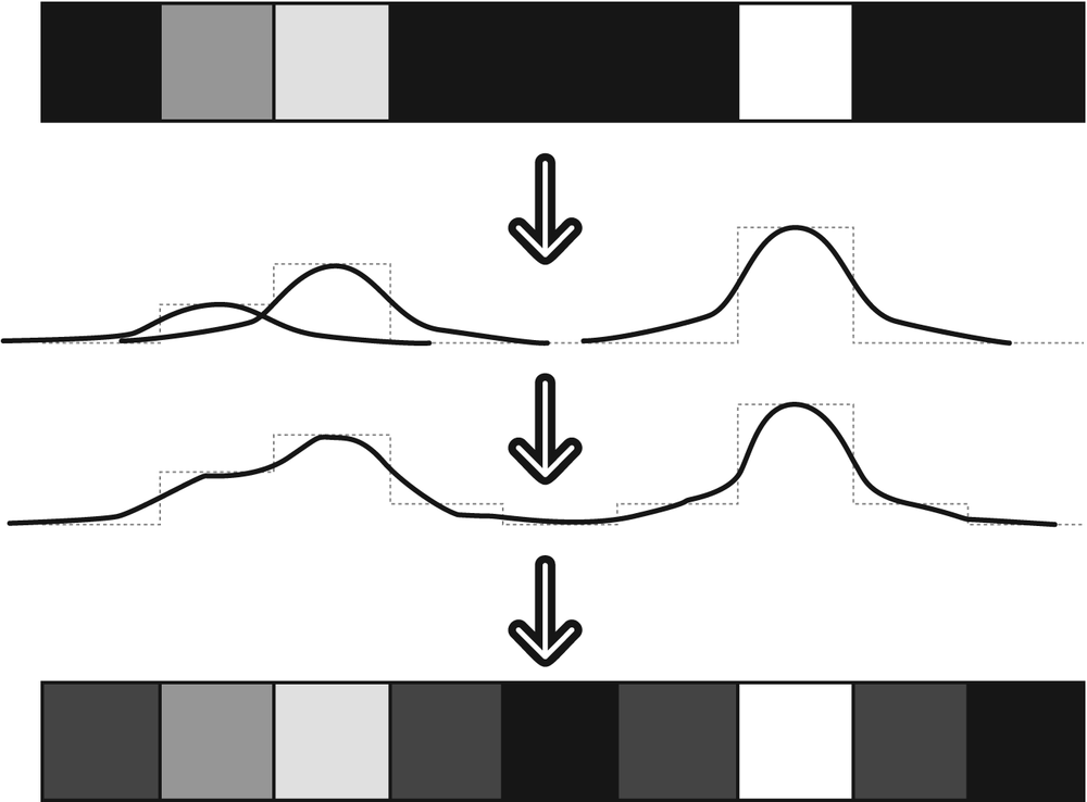
The simple blur operation, as exemplified by
CV_BLUR in Figure 5-1, is the simplest case. Each pixel in
the output is the simple mean of all of the pixels in a window around the corresponding
pixel in the input. Simple blur supports any number of channels and works on 8-bit images or
32-bit floating-point images.
Not all of the smoothing operators act on the same sorts of images. CV_BLUR_NO_SCALE (simple blur without
scaling) is essentially the same as simple blur except that there is no
division performed to create an average. Hence the source and destination images must have
different numerical precision so that the blurring operation will not result in an overflow.
Simple blur without scaling may be performed on 8-bit images, in which case the destination
image should have IPL_DEPTH_16S (CV_16S) or IPL_DEPTH_32S (CV_32S) data types. The same operation may also
be performed on 32-bit floating-point images, in which case the destination image may also
be a 32-bit floating-point image. Simple blur without scaling cannot be done in place: the
source and destination images must be different. (This requirement is obvious in the case of
8 bits to 16 bits, but it applies even when you are using a 32-bit image). Simple blur
without scaling is sometimes chosen because it is a little faster than blurring with
scaling.

Figure 5-1. Image smoothing by block averaging: on the left are the input images; on the right, the output images
The median filter (CV_MEDIAN) [Bardyn84] replaces each pixel by the median or "middle" pixel (as
opposed to the mean pixel) value in a square neighborhood around the center pixel.
Median filter will work on single-channel or three-channel or four-channel 8-bit
images, but it cannot be done in place. Results of median filtering are shown in Figure 5-2. Simple blurring by averaging can be
sensitive to noisy images, especially images with large isolated outlier points (sometimes
called "shot noise"). Large differences in even a small number of points can cause a
noticeable movement in the average value. Median filtering is able to ignore the outliers by
selecting the middle points.
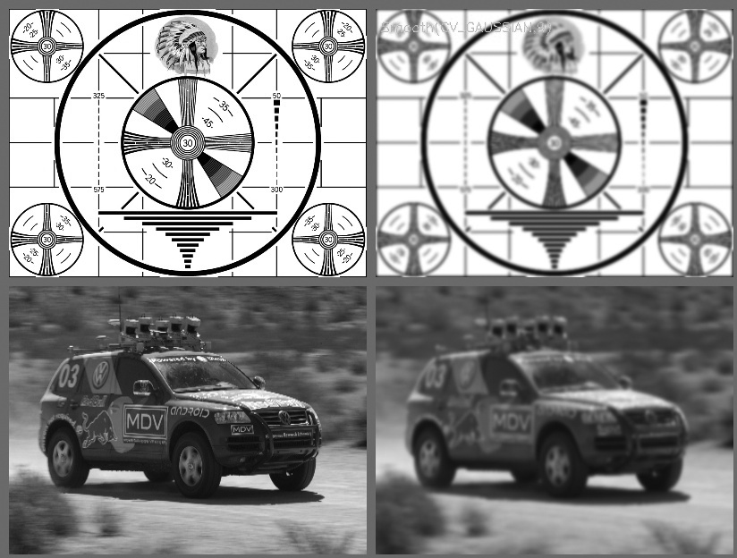
The next smoothing filter, the Gaussian filter
(CV_GAUSSIAN), is probably the most useful though not
the fastest. Gaussian filtering is done by convolving each point in the input array with a
Gaussian kernel and then summing to produce the output array.

For the Gaussian blur (Figure 5-3), the first two parameters give the width and height of the filter window; the (optional) third parameter indicates the sigma value (half width at half max) of the Gaussian kernel. If the third parameter is not specified, then the Gaussian will be automatically determined from the window size using the following formulae:

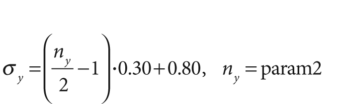
If you wish the kernel to be asymmetric, then you may also (optionally) supply a fourth parameter; in this case, the third and fourth parameters will be the values of sigma in the horizontal and vertical directions, respectively.
If the third and fourth parameters are given but the first two are set to 0, then the size of the window will be automatically determined from the value of sigma.
The OpenCV implementation of Gaussian smoothing also provides a higher performance optimization for several common kernels. 3-by-3, 5-by-5 and 7-by-7 with the "standard" sigma (i.e., param3 = 0.0) give better performance than other kernels. Gaussian blur supports single- or three-channel images in either 8-bit or 32-bit floating-point formats, and it can be done in place. Results of Gaussian blurring are shown in Figure 5-4.
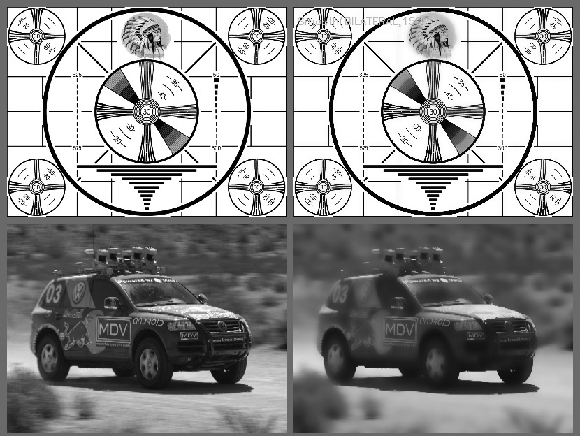
The fifth and final form of smoothing supported by OpenCV is called bilateral filtering [Tomasi98], an example of which is shown in Figure 5-5. Bilateral filtering is one operation from a somewhat larger class of image analysis operators known as edge-preserving smoothing. Bilateral filtering is most easily understood when contrasted to Gaussian smoothing. A typical motivation for Gaussian smoothing is that pixels in a real image should vary slowly over space and thus be correlated to their neighbors, whereas random noise can be expected to vary greatly from one pixel to the next (i.e., noise is not spatially correlated). It is in this sense that Gaussian smoothing reduces noise while preserving signal. Unfortunately, this method breaks down near edges, where you do expect pixels to be uncorrelated with their neighbors. Thus Gaussian smoothing smoothes away the edges. At the cost of a little more processing time, bilateral filtering provides us a means of smoothing an image without smoothing away the edges.
Like Gaussian smoothing, bilateral filtering constructs a weighted average of each pixel and its neighboring components. The weighting has two components, the first of which is the same weighting used by Gaussian smoothing. The second component is also a Gaussian weighting but is based not on the spatial distance from the center pixel but rather on the difference in intensity[48] from the center pixel.[49]You can think of bilateral filtering as Gaussian smoothing that weights more similar pixels more highly than less similar ones. The effect of this filter is typically to turn an image into what appears to be a watercolor painting of the same scene.[50] This can be useful as an aid to segmenting the image.
Bilateral filtering takes two parameters. The first is the width of the Gaussian kernel used in the spatial domain, which is analogous to the sigma parameters in the Gaussian filter. The second is the width of the Gaussian kernel in the color domain. The larger this second parameter is, the broader is the range of intensities (or colors) that will be included in the smoothing (and thus the more extreme a discontinuity must be in order to be preserved).
[46] Note that—unlike in, say, Matlab—the filtering operations in OpenCV (e.g., cvSmooth(), cvErode(), cvDilate()) produce output images of the same size
as the input. To achieve that result, OpenCV creates "virtual" pixels outside of the image at the borders. By default, this is done by
replication at the border, i.e., input(-dx,y)=input(0,y),
input(w+dx,y)=input(w-1,y), and so forth.
[47] Here and elsewhere we sometimes use 8u as shorthand for 8-bit unsigned image depth
(IPL_DEPTH_8U). See Table 3-2 for other shorthand notation.
[48] In the case of multichannel (i.e., color) images, the difference in intensity is replaced with a weighted sum over colors. This weighting is chosen to enforce a Euclidean distance in the CIE color space.
[49] Technically, the use of Gaussian distribution functions is not a necessary feature of bilateral filtering. The implementation in OpenCV uses Gaussian weighting even though the method is general to many possible weighting functions.
[50] This effect is particularly pronounced after multiple iterations of bilateral filtering.