Canny

The method just described for finding edges was further refined by J. Canny in 1986 into what is now commonly called the Canny edge detector [Canny86]. One of the differences between the Canny algorithm and the simpler, Laplace-based algorithm from the previous section is that, in the Canny algorithm, the first derivatives are computed in x and y and then combined into four directional derivatives. The points where these directional derivatives are local maxima are then candidates for assembling into edges.

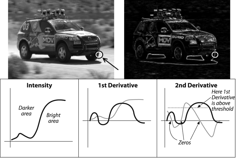
Figure 6-6. Laplace transform (upper right) of the racecar image: zooming in on the tire (circled in white) and considering only the x-dimension, we show a (qualitative) representation of the brightness as well as the first and second derivative (lower three cells); the 0s in the second derivative correspond to edges, and the 0 corresponding to a large first derivative is a strong edge

However, the most significant new dimension to the Canny algorithm is that it tries to assemble the individual edge candidate pixels into contours. ^[67] These contours are formed by applying an hysteresis threshold to the pixels. This means that there are two thresholds, an upper and a lower. If a pixel has a gradient larger than the upper threshold, then it is accepted as an edge pixel; if a pixel is below the lower threshold, it is rejected. If the pixel's gradient is between the thresholds, then it will be accepted only if it is connected to a pixel that is above the high threshold. 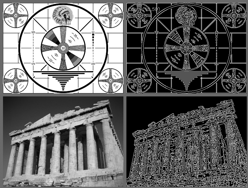Canny recommended a ratio of high:low threshold between 2:1 and 3:1. Figures Figure 6-7 and Figure 6-8 show the results of applying cvCanny() to a test pattern and a photograph using high:low hysteresis threshold ratios of 5:1 and 3:2, respectively.

void cvCanny(
   const CvArr*  img,
   CvArr*        edges,
   double        lowThresh,
   double        highThresh,
   int           apertureSize = 3
);

Figure 6-7. Results of Canny edge detection for two different images when the high and low thresholds are set to 50 and 10, respectively

The cvCanny() function expects an input image, which must be grayscale, and an output image, which must also be grayscale (but which will actually be a Boolean image). The next two arguments are the low and high thresholds, and the last argument is another aperture. As usual, this is the aperture used by the Sobel derivative operators that are called inside of the implementation of cvCanny().

---

^[67] We'll have much more to say about contours later. As you await those revelations, though, keep in mind that the cvCanny() routine does not actually return objects of type CvContour; we will have to build those from the output of cvCanny() if we want them by using cvFindContours(). Everything you ever wanted to know about contours will be covered in Chapter 8.