We will go through decision trees in detail, since they are highly useful and use most of the functionality in the machine learning library (and thus serve well as an instructional example). Binary decision trees were invented by Leo Breiman and colleagues,[245] who named them classification and regression tree (CART) algorithms. This is the decision tree algorithm that OpenCV implements. The gist of the algorithm is to define an impurity metric relative to the data in every node of the tree. For example, when using regression to fit a function, we might use the sum of squared differences between the true value and the predicted value. We want to minimize the sum of differences (the "impurity") in each node of the tree. For categorical labels, we define a measure that is minimal when most values in a node are of the same class. Three common measures to use are entropy, Gini index, and misclassification (all are described in this section). Once we have such a metric, a binary decision tree searches through the feature vector to find which feature combined with which threshold most purifies the data. By convention, we say that features above the threshold are "true" and that the data thus classified will branch to the left; the other data points branch right. This procedure is then used recursively down each branch of the tree until the data is of sufficient purity or until the number of data points in a node reaches a set minimum.
The equations for node impurity i(N) are given next. We must deal with two cases, regression and classification.
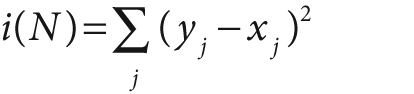
For regression or function fitting, the equation for node impurity is simply the square of the difference in value between the node value y and the data value x. We want to minimize:
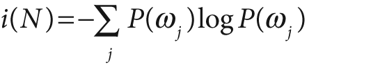
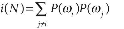
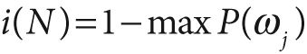
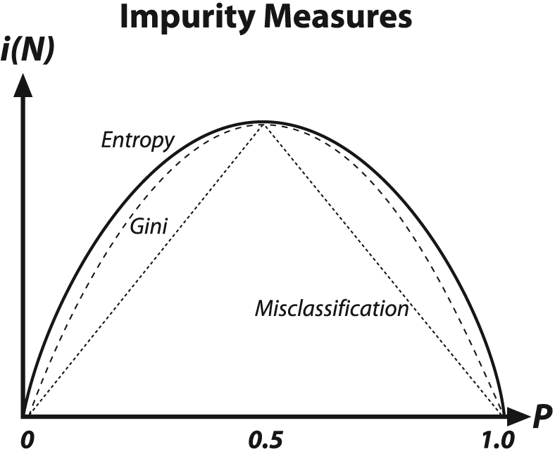
For classification, decision trees often use one of three methods: entropy impurity, Gini impurity, or misclassification impurity. For these methods, we use the notation P(ωj) to denote the fraction of patterns at node N that are in class ωj. Each of these impurities has slightly different effects on the splitting decision. Gini is the most commonly used, but all the algorithms attempt to minimize the impurity at a node. Figure 13-7 graphs the impurity measures that we want to minimize.
Decision trees are perhaps the most widely used classification technology. This is due to their simplicity of implementation, ease of interpretation of results, flexibility with different data types (categorical, numerical, unnormalized and mixes thereof), ability to handle missing data through surrogate splits, and natural way of assigning importance to the data features by order of splitting. Decision trees form the basis of other algorithms such as boosting and random trees, which we will discuss shortly.
In what follows we describe perhaps more than enough for you to get decision trees
working well. However, there are many more methods for accessing nodes, modifying splits,
and so forth. For that level of detail (which few readers are likely ever to need) you
should consult the user manual …/opencv/docs/ref/opencvref_ml.htm, particularly with regard to the classes
CvDTree{}, the training class CvDTreeTrainData{}, and the nodes CvDTreeNode{} and splits
CvDTreeSplit{}.
For a pragmatic introduction, we start by dissecting a specific example. In the
…/opencv/samples/c directory, there is a mushroom.cpp file that runs decision trees on the agaricus-lepiota.data data file. This data file consists of a
label "p" or "e" (denoting poisonous or edible, respectively) followed by 22 categorical attributes, each represented
by a single letter. Observe that the data file is given in "comma separated value" (CSV)
format, where the features' values are separated from each other by commas. In mushroom.cpp there is a rather messy function mushroom_read_database() for reading in this particular data
file. This function is rather overspecific and brittle but mainly it's just filling three
arrays as follows. (1) A floating-point matrix data[][], which has dimensions rows = number of data points by columns = number
of features (22 in this case) and where all the features are converted from their
categorical letter values to floating-point numbers. (2) A character matrix missing[][], where a "true" or "1" indicates a missing value
that is indicated in the raw data file by a question mark and where all other values are
set to 0. (3) A floating-point vector responses[],
which contains the poison "p" or edible "e" response cast in floating-point values. In
most cases you would write a more general data input program. We'll now discuss the main
working points of mushroom.cpp, all of which are
called directly or indirectly from main() in the
program.
For training the tree, we fill out the tree parameter structure CvDTreeParams{}:
struct CvDTreeParams {

  int   max_categories;       //Until pre-clustering
  int   max_depth;            //Maximum levels in a tree
  int   min_sample_count;     //Don't split a node if less
  int   cv_folds;             //Prune tree with K fold cross-validation
  bool  use_surrogates;       //Alternate splits for missing data
  bool  use_1se_rule;         //Harsher pruning
  bool  truncate_pruned_tree; //Don't "remember" pruned branches
  float regression_accuracy;  //One of the "stop splitting" criteria
  const float* priors;        //Weight of each prediction category

  CvDTreeParams() : max_categories(10), max_depth(INT_MAX),
    min_sample_count(10), cv_folds(10), use_surrogates(true),
    use_1se_rule(true), truncate_pruned_tree(true),
    regression_accuracy(0.01f), priors(NULL) { ; }

  CvDTreeParams(
    int          _max_depth,
    int          _min_sample_count,
    float        _regression_accuracy,
    bool         _use_surrogates,
    int          _max_categories,
    int          _cv_folds,
    bool         _use_1se_rule,
    bool         _truncate_pruned_tree,
    const float* _priors
  );
}
In the structure, max_categories has a default
value of 10. This limits the number of categorical values before which the decision tree
will precluster those categories so that it will have to test no more than 2
max_categories
–2 possible value subsets.[246] This isn't a problem for ordered or numerical features, where the algorithm
just has to find a threshold at which to split left or right. Those variables that have
more categories than max_categories will have their
category values clustered down to max_categories
possible values. In this way, decision trees will have to test no more than max_categories levels at a time. This parameter, when set to
a low value, reduces computation at the cost of accuracy.
The other parameters are fairly self-explanatory. The last parameter, priors, can be crucial. It sets the relative weight that you
give to misclassification. That is, if the weight of the first category is 1 and the
weight of the second category is 10, then each mistake in predicting the second category
is equivalent to making 10 mistakes in predicting the first category. In the code we
have edible and poisonous mushrooms, so we "punish" mistaking a poisonous
mushroom for an edible one 10 times more than mistaking an edible mushroom for a
poisonous one.
The template of the methods for training a decision tree is shown below. There are two methods: the first is used for working directly with decision trees; the second is for ensembles (as used in boosting) or forests (as used in random trees).
// Work directly with decision trees:
  bool CvDTree::train(
  const CvMat*  _train_data,
  int           _tflag,
  const CvMat*  _responses,
  const CvMat*  _var_idx      = 0,
  const CvMat*  _sample_idx   = 0,
  const CvMat*  _var_type     = 0,
  const CvMat*  _missing_mask = 0,
  CvDTreeParams params        = CvDTreeParams()
);

// Method that ensembles of decision trees use to call individual

// training for each tree in the ensemble
bool CvDTree::train(
  CvDTreeTrainData* _train_data,
  const CvMat*      _subsample_idx
);
In the train() method, we have the floating-point
_train_data[][] matrix. In that matrix, if _tflag is set to CV_ROW_SAMPLE then each row is a data point consisting of a vector of
features that make up the columns of the matrix. If tflag is set to CV_COL_SAMPLE, the row
and column meanings are reversed. The _responses[]
argument is a floating-point vector of values to be predicted given the data features.
The other parameters are optional. The vector _var_idx indicates features to include, and the vector _sample_idx indicates data points to include; both of these
vectors are either zero-based integer lists of values to skip or 8-bit masks of active
(1) or skip (0) values (see our general discussion of the train() method earlier in the chapter). The byte (CV_8UC1) vector _var_type is a
zero-based mask for each feature type (CV_VAR_CATEGORICAL or CV_VAR_ORDERED[247]); its size is equal to the number of features plus 1. That last entry is for
the response type to be learned. The byte-valued _missing_mask[][] matrix is used to indicate missing values with a 1 (else
0 is used). Example 13-2 details the creation
and training of a decision tree.
Example 13-2. Creating and training a decision tree
float priors[] = { 1.0, 10.0}; // Edible vs poisonous weights

CvMat* var_type;

var_type = cvCreateMat( data->cols + 1, 1, CV_8U );

cvSet( var_type, cvScalarAll(CV_VAR_CATEGORICAL) ); // all these vars
                                                    // are categorical
CvDTree* dtree;
dtree = new CvDTree;
dtree->train(
  data,
  CV_ROW_SAMPLE,
  responses,
  0,
  0,
  var_type,
  missing,
  CvDTreeParams(
    8,     // max depth
    10,    // min sample count
    0,     // regression accuracy: N/A here
    true,  // compute surrogate split,
           //   since we have missing data
    15,    // max number of categories
           //   (use suboptimal algorithm for
           //   larger numbers)
    10,    // cross-validations
    true,  // use 1SE rule => smaller tree
    true,  // throw away the pruned tree branches
    priors // the array of priors, the bigger
           //   p_weight, the more attention
           //   to the poisonous mushrooms
  )
);
In this code the decision tree dtree is declared
and allocated. The dtree->train()
method is then called. In this case, the vector of responses[] (poisonous or edible) was set to the ASCII value of "p" or "e" (respectively) for each
data point. After the train() method terminates,
dtree is ready to be used for predicting new data. The decision tree may also be saved to disk via
save() and loaded via load() (each method is shown below).[248] Between the saving and the loading, we reset and zero out the tree by
calling the clear() method.
dtree->save("tree.xml","MyTree");

dtree->clear();

dtree->load("tree.xml","MyTree");
This saves and loads a tree file called tree.xml. (Using the .xml extension
stores an XML data file; if we used a .yml or
.yaml extension, it would store a YAML data
file.) The optional "MyTree" is a tag that labels the
tree within the tree.xml file. As with other
statistical models in the machine learning module, multiple objects cannot be stored in
a single .xml or .yml file when using save(); for
multiple storage one needs to use cvOpenFileStorage()
and write(). However, load() is a different story: this function can load an object by its name
even if there is some other data stored in the file.
The function for prediction with a decision tree is:
CvDTreeNode* CvDTree::predict(
  const CvMat* _sample,
  const CvMat* _missing_data_mask = 0,
  bool         raw_mode           = false
) const;
Here _sample is a floating-point vector of
features used to predict; _missing_data_mask is a
byte vector of the same length and orientation[249] as the _sample vector, in which nonzero
values indicate a missing feature value. Finally, raw_mode indicates unnormalized data with "false" (the default) or "true"
for normalized input categorical data values. This is mainly used in ensembles of trees
to speed up prediction. Normalizing data to fit within the (0, 1) interval is simply a
computational speedup because the algorithm then knows the bounds in which data may
fluctuate. Such normalization has no effect on accuracy. This method returns a node of
the decision tree, and you may access the predicted value using (CvDTreeNode *)->value which is returned by the dtree->predict() method (see CvDTree::predict() described previously):
double r = dtree->predict( &sample, &mask )->value;
Finally, we can call the useful var_importance()
method to learn about the importance of the individual features. This function will
return an N-by-1 vector of type double (CV_64FC1) containing each feature's relative importance for prediction,
where the value 1 indicates the highest importance and 0 indicates absolutely not important or useful for prediction.
Unimportant features may be eliminated on a second-pass training. (See Figure 13-12 for a display of variable importance.) The call is as follows:
const CvMat* var_importance = dtree->get_var_importance();
As demonstrated in the …/opencv/samples/c/mushroom.cpp file, individual elements of the importance vector may be accessed directly via
double val = var_importance->data.db[i];
Most users will only train and use the decision trees, but advanced or research
users may sometimes wish to examine and/or modify the tree nodes or the splitting
criteria. As stated in the beginning of this section, the information for how to do this
is in the ML documentation that ships with OpenCV at …/opencv/docs/ref/opencvref_ml.htm#ch_dtree, which can also be accessed
via the OpenCV Wiki (http://opencvlibrary.sourceforge.net/). The sections
of interest for such advanced analysis are the class structure CvDTree{}, the training structure CvDTreeTrainData{}, the node structure CvDTreeNode{}, and its contained split structure CvDTreeSplit{}.
Using the code just described, we can learn several things about edible or poisonous mushrooms from the agaricus-lepiota.data file. If we just train a decision tree without pruning, so that it learns the data perfectly, we get the tree shown in Figure 13-8. Although the full decision tree learns the training set of data perfectly, remember the lesson of Figure 13-2 (overfitting). What we've done in Figure 13-8 is to memorize the data together with its mistakes and noise. Thus, it is unlikely to perform well on real data. That is why OpenCV decision trees and CART type trees typically include an additional step of penalizing complex trees and pruning them back until complexity is in balance with performance. There are other decision tree implementations that grow the tree only until complexity is balanced with performance and so combine the pruning phase with the learning phase. However, during development of the ML library it was found that trees that are fully grown first and then pruned (as implemented in OpenCV) performed better than those that combine training with pruning in their generation phase.
Figure 13-9 shows a pruned tree that
still does quite well (but not perfectly) on the training set but will probably perform
better on real data because it has a better balance between bias and variance. Yet this
classifier has an serious shortcoming: Although it performs well on the data, it still
labels poisonous mushrooms as edible 1.23% of the time. Perhaps we'd be happier with a
worse classifier that labeled many edible mushrooms as poisonous provided it never invited us to eat a poisonous
mushroom! Such a classifier can be created by intentionally biasing the classifier and/or the data. This is sometimes
referred to as adding a cost to the classifier. In our case, we want
to add a higher cost for misclassifying poisonous mushrooms than for misclassifying
edible mushrooms. Cost can be imposed "inside" a classifier by changing the
weighting of how much a "bad" data point counts versus a "good" one. OpenCV allows you to
do this by adjusting the priors vector in the CvDTreeParams{} structure passed to the train() method, as we have discussed previously. Even without
going inside the classifier code, we can impose a prior cost by duplicating (or resampling
from) "bad" data. Duplicating "bad" data points implicitly gives a higher weight to the
"bad" data, a technique that can work with any classifier.
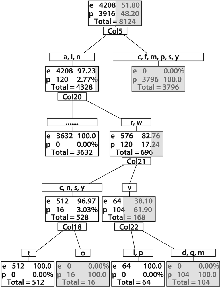
Figure 13-8. Full decision tree for poisonous (p) or edible (e) mushrooms: this tree was built out to full complexity for 0% error on the training set and so would probably suffer from variance problems on test or real data (the dark portion of a rectangle represents the poisonous portion of mushrooms at that phase of categorization)
Figure 13-10 shows a tree where a 10 X bias was imposed against poisonous mushrooms. This tree makes no mistakes on poisonous mushrooms at a cost of many more mistakes on edible mushrooms'a case of "better safe than sorry". Confusion matrices for the (pruned) unbiased and biased trees are shown in Figure 13-11.
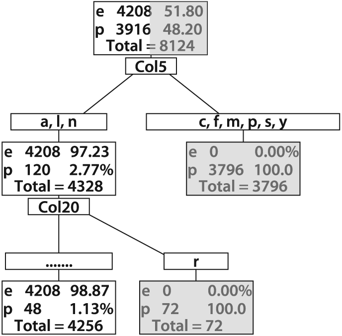
Figure 13-9. Pruned decision tree for poisonous (p) and edible (e) mushrooms: despite being pruned, this tree shows low error on the training set and would likely work well on real data
Figure 13-10. An edible mushroom decision tree with 10 × bias against misidentification of poisonous mushrooms as edible; note that the lower right rectangle, though containing a vast majority of edible mushrooms, does not contain a 10 × majority and so would be classified as inedible
Finally, we can learn something more from the data by using the variable importance machinery that comes with the tree-based classifiers in OpenCV.[250] Variable importance measurement techniques were discussed in a previous subsection, and they involve successively perturbing each feature and then measuring the effect on classifier performance. Features that cause larger drops in performance when perturbed are more important. Also, decision trees directly show importance via the splits they found in the data: the first splits are presumably more important than later splits. Splits can be a useful indicator of importance, but they are done in a "greedy" fashion—finding which split most purifies the data now. It is often the case that doing a worse split first leads to better splits later, but these trees won't find this out.[251] The variable importance for poisonous mushrooms is shown in Figure 13-12 for both the unbiased and the biased trees. Note that the order of important variables changes depending on the bias of the trees.
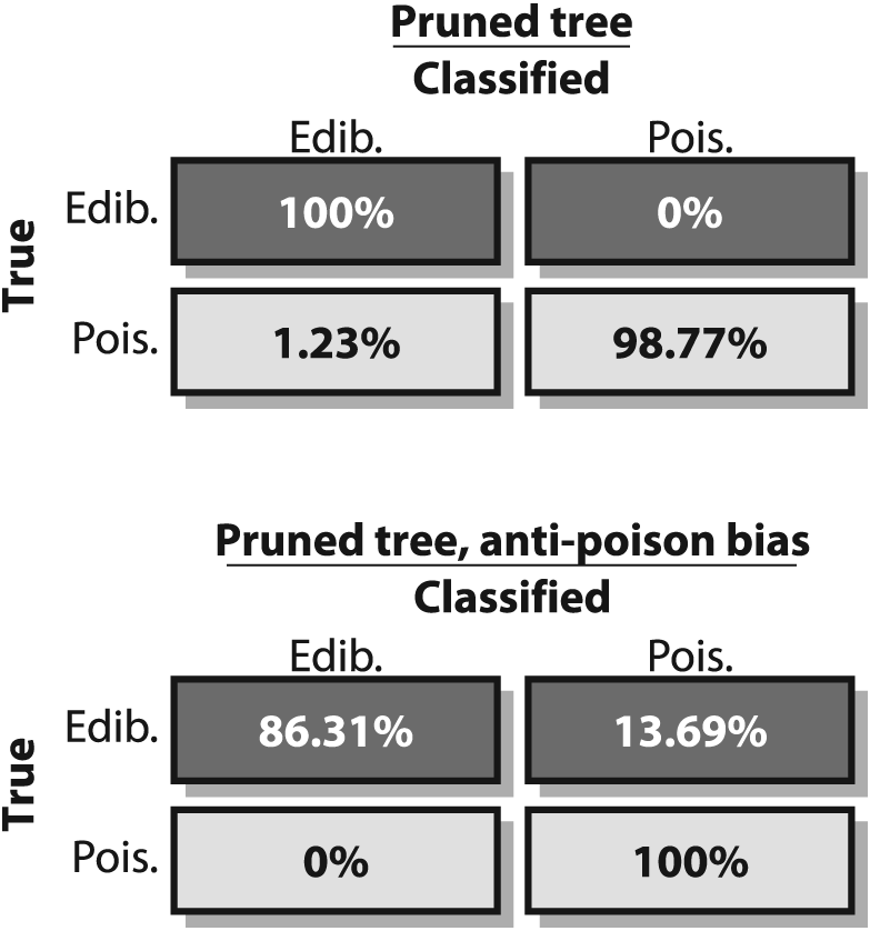
Figure 13-11. Confusion matrices for (pruned) edible mushroom decision trees: the unbiased tree yields better overall performance (top panel) but sometimes misclassifies poisonous mushrooms as edible; the biased tree does not perform as well overall (lower panel) but never misclassifies poisonous mushrooms
[245] L. Breiman, J. Friedman, R. Olshen, and C. Stone, Classification and Regression Trees (1984), Wadsworth.
[246] More detail on categorical vs. ordered splits: Whereas a split on an ordered
variable has the form "if x < a then go left, else go
right", a split on a categorical variable has the form "if 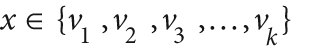 then go left, else go right", where the
vi are some possible values of the
variable. Thus, if a categorical variable has N possible values
then, in order to find a best split on that variable, one needs to try
2
N
–2 subsets (empty and full subset are excluded). Thus, an approximate algorithm is used
whereby all N values are grouped into K ≤
then go left, else go right", where the
vi are some possible values of the
variable. Thus, if a categorical variable has N possible values
then, in order to find a best split on that variable, one needs to try
2
N
–2 subsets (empty and full subset are excluded). Thus, an approximate algorithm is used
whereby all N values are grouped into K ≤
max_categories clusters (via the K-mean
algorithm) based on the statistics of the samples in the currently analyzed node.
Thereafter, the algorithm tries different combinations of the clusters and chooses
the best split, which often gives quite a good result. Note that for the two most
common tasks, two-class classification and regression, the optimal categorical split
(i.e., the best subset of values) can be found efficiently without any clustering.
Hence the clustering is applied only in n > 2-class
classification problems for categorical variables with N >
max_categories possible values. Therefore, you
should think twice before setting max_categories
to anything greater than 20, which would imply more than a million operations for
each split!
[247] CV_VAR_ORDERED is the same thing as CV_VAR_NUMERICAL.
[248] As mentioned previously, save() and load() are convenience wrappers for the more complex
functions write() and read().
[249] By "same … orientation" we mean that if the sample is a 1-by-N vector the mask must be 1-by-N, and if the sample is N-by-1 then the mask must be N-by-1.
[250] Variable importance techniques may be used with any classifier, but at this time OpenCV implements them only with tree-based methods.
[251] OpenCV (following Breiman's technique) computes variable importance across all the splits, including surrogate ones, which decreases the possible negative effect that CART's greedy splitting algorithm would have on variable importance ratings.