Applying Backpropagation
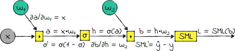
Here is our three-layered network, in the form of a computational graph:
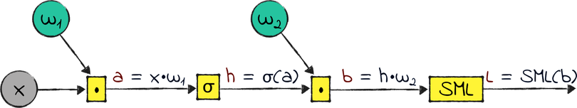
All the variables in the preceding graph are matrices, with the exception of the loss L. The σ symbol represents the sigmoid. For reasons that will become clear in a minute, I squashed the softmax and the cross-entropy loss into one operation. I needed a name for that operation, so I temporarily called it SML, for “softmax and loss.” Finally, I gave the names a and b to the outputs of the matrix multiplications.
The diagram shown earlier represents the same neural network that we designed and built in the previous two chapters. Follow its operations from left to right: x and w₁ get multiplied and passed through the sigmoid, producing the hidden layer h; then, h is multiplied by w₂ and passed through the softmax and the loss function, producing the loss L.
Now let’s come to the reason we learned backpropagation: we want to calculate the gradients of L with respect to w₁ and w₂. To apply the chain rule, we need the local gradients on the paths back from L to w₁ and w₂:
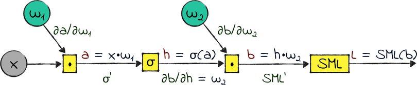
σ’ and SML’ are the derivatives of the sigmoid and the SML operation, respectively. In most of this book I used names such as ∂σ/∂a to indicate derivatives—but if a function has only one variable, as in these cases, then you can indicate its derivative with a simple apostrophe.
Let’s roll up our sleeves and calculate those local gradients. Once again, you don’t need to be able to take those derivatives on your own. That’s what I’m here for! Here are the results:
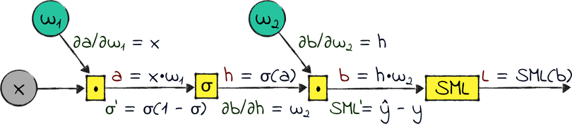
Back in Cross Entropy, I said that the softmax and the cross-entropy loss are a perfect match. Now we can see why. Taken separately, those functions have complicated derivatives—but compose them, and their derivative boils down to a simple formula that’s cheap to compute: the network’s output minus the ground truth. If you want to see the math behind this derivative, you can find a step-by-step explanation on the ProgML[18] site.
The derivatives of the matrix multiplications are also short and sweet. If you know how to calculate the derivative of scalar multiplication—well, the derivative of matrix multiplication is the same.
Finally, I looked up the sigmoid’s derivative in a math textbook. It’s a peculiar one, because it’s expressed in terms of the sigmoid itself.
Now that we have the local gradients, we can apply the chain rule to calculate the gradients of the weights. This time, however, we’re not going to do it on paper—we’re going to write code.
Staying the Course
We’re about to write a backpropagation function that calculates the gradients of the weights in our neural network. Here is a word of warning before we begin: this function is going to be short, but complicated.
We will write code that’s a direct application of the chain rule. The chain rule is straightforward when you apply it to scalar gradients, but gets tricky with matrices. In a neural network, you have to “make the multiplications work” by swapping and transposing the operands, so that the dimensions of the matrices involved work well together.
That juggling of matrices is actually easier to do than it is to describe. When you write your own backprop code, you can double-check your calculations in an interpreter, and use the matrix dimensions as a guideline to decide which matrices to transpose, in which order to multiply them, and so on. In written form, however, the reasoning behind those operations takes up more space than we have available in this chapter.
All those things considered, now you have a few options:
-
You can read through the rest of this section and see how the backprop code comes together, breezing over the twisty details.
-
You can go through the next few pages more carefully, double-checking the matrix operations on your own, either on paper or in a Python interpreter.
-
If you’re looking for some hard work, you can even write the backpropagation code yourself, peeking at the next pages for hints if you get stuck. This last option is challenging, but it’s the best way to wrap your head around all the details of this code, if you’re so inclined.
Whichever option you choose, don’t get discouraged if you struggle through the corner cases in the next two pages. Those corner cases aren’t the point of this chapter. The point is to understand the idea behind backpropagation, and how this code came together.
Preamble done. Let’s write the code that calculates the gradient of w₂.
Calculating the Gradient of w₂
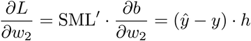
Here are the local gradients involved in the calculation of ∂L/∂w₂:
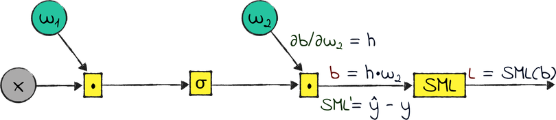
Apply the chain rule with an eye on the previous diagram and you get:
And here is that formula turned to code:
| | w2_gradient = np.matmul(prepend_bias(h).T, y_hat - Y) / X.shape[0] |
I had to swap the operands of the multiplication, and transpose one of them—all in the interest of getting a result with the same dimensions as w₂. Remember that we’re going to multiply this gradient by the learning rate, and subtract it from w₂, so the two matrices must have the same shape.
This one-liner contains two more details that you might find baffling. One is the call to prepend_bias. To make sense of it, remember that in the forward function, we add a bias column to h, so we need to do the same during backprop.
The second perplexing detail is the division by X.shape[0] at the end. That’s the number of rows in X—that is, the number of examples in the training set. This division is there because the matrix multiplication gives us the accumulated gradient over all the examples. Because we want the average gradient, we have to divide the result of the multiplication by the size of the training set.
That was a tightly packed line of code. On to the gradient of w₁!
Calculating the Gradient of w₁
Let’s look at the local gradients that we need to calculate ∂L/∂w₁:
Here comes the chain rule:

That’s a long formula. I split it over two lines of code and a helper function:
| | def sigmoid_gradient(sigmoid): |
| | return np.multiply(sigmoid, (1 - sigmoid)) |
| | a_gradient = np.matmul(y_hat - Y, w2[1:].T) * sigmoid_gradient(h) |
| | w1_gradient = np.matmul(prepend_bias(X).T, a_gradient) / X.shape[0] |
The next-to-last line calculates ![]() . There are a few subtleties involved in this calculation. To begin with, this time around we’re using h as is, without a bias column. Fact is, the bias column gets added after the calculation of h, so its gradient doesn’t propagate as far back as the gradient of w1. In other words, that column has no effect on ∂L/∂w₁.
. There are a few subtleties involved in this calculation. To begin with, this time around we’re using h as is, without a bias column. Fact is, the bias column gets added after the calculation of h, so its gradient doesn’t propagate as far back as the gradient of w1. In other words, that column has no effect on ∂L/∂w₁.
Now, here’s a twist: because we ignored the first column of h, we also have to ignore its weights. That’s the first row of w2, because matrix multiplication matches columns by rows. That’s what w2[1:] means: “w2, without the first row.”
I have to admit that I got this code wrong the first time. After NumPy complained that my matrix dimensions didn’t match, I fixed the code by thinking through the dimensions of all the matrices involved. It was a pretty painful experience.
Moving on with this line of code: the sigmoid_gradient helper function calculates the sigmoid’s gradient from the sigmoid’s output. We already know that the sigmoid’s output is the hidden layer h, so we can just call sigmoid_gradient(h).
The last line in the code finishes the job, multiplying the previous intermediate result by X. This multiplication involves the same trickery that we experienced when we calculated the gradient of w₂: we need to swap the operands, transpose one of the matrices, prepend the bias column to X like we do during forward propagation, and average the final gradient over the training examples.
Phew! I told you that this code was going to be tricky, but we’re done now. We can put it all together.
Distilling the back Function
Here is the backpropagation code, inlined and wrapped into a convenient three-lines function:
| | def back(X, Y, y_hat, w2, h): |
| | w2_gradient = np.matmul(prepend_bias(h).T, (y_hat - Y)) / X.shape[0] |
| | w1_gradient = np.matmul(prepend_bias(X).T, np.matmul(y_hat - Y, w2[1:].T) |
| | * sigmoid_gradient(h)) / X.shape[0] |
| | return (w1_gradient, w2_gradient) |
Congratulations! We’re done writing the hardest piece of code in this book.
Now that we have the back function, we’re one big step closer to a fully functioning GD algorithm for our neural network. We just need to take care of one last detail: before we start tuning the weights, we have to initialize them. That matter deserves its own section.