Understanding Activation Functions
By now, you’re familiar with activation functions—those cyan boxes in between a neural network’s layers shown in the diagram.
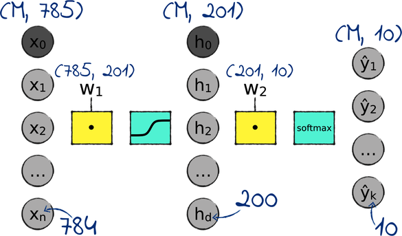
All our activation functions so far have been sigmoids, except in the output layer, where we used the softmax function.
The sigmoid has been with us for a long time. I originally introduced it to squash the output of a perceptron so that it ranged from 0 to 1. Later on, I introduced the softmax to rescale a neural network’s outputs so that they added up to 1. By rescaling the outputs, we could interpret them as probabilities, as in: “we have a 30% chance that this picture contains a platypus.”
Now that we’re building deep neural networks, however, those original motivations feel so far away. Activation functions complicate our neural networks, and they don’t seem to give us much in exchange. Can’t we just get rid of them?
What Activation Functions Are For
Let’s see what happens if we remove the activation functions from a neural network. Here is the network we just saw, minus the activation functions:
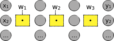
This network sure looks simpler than the earlier one. However, it comes with a crippling limitation: all its operations are linear, meaning that they could be plotted with straight shapes. To explore the consequences of this linearity, let’s work through a tiny bit of math.
In a network without activation functions, each of the n layers is the weighted sum of the nodes in the previous layer:
![]()
![]()
…
![]()
We can squash all those formulae together and calculate the last layer as the multiplication of the first layer with all the weight matrices in between:
![]()
Now, here’s the twist: If you take all those matrix multiplications of weights and call them w, the previous formula boils down to:
![]()
In other words, we just reduced the entire neural network to a single weighted sum:
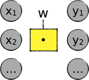
We came to a pretty stark result: No matter how many linear operations we pile up, they always add up to a single linear operation. In concrete terms, a network where everything is linear collapses to a feeble linear regression program, like the one we wrote in Chapter 4, Hyperspace!.
Activation functions prevent that collapse because they’re nonlinear—that is, they cannot be plotted as straight shapes. That nonlinearity is the heart and soul of a neural network.
You just learned that nonlinear activation functions are essential. However, that doesn’t mean that we’re stuck with the sigmoid and the softmax. We can replace them with other nonlinear functions—and in the case of the sigmoid, in particular, that might be a good idea. Let’s see why.
The Sigmoid and Its Consequences
Say hello to our old friend, the sigmoid, shown in the graph that follows:
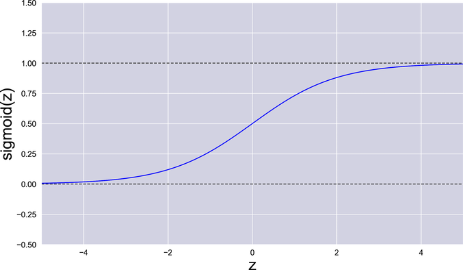
You just learned that an activation function should be nonlinear—that is, non-straight. The curvy sigmoid fits that bill.
At first sight, the sigmoid also jives well with backpropagation. Remember the chain rule? The global gradient of the neural network is the product of the local gradients of its components. The sigmoid contributes a local gradient that’s nice and smooth. Slide your finger along its curve, and you’ll find no hole, cusp, or sudden jump that can trip up gradient descent.
Look closer, however, and the sigmoid begins to reveal its shortcomings. Let’s talk about them.
Dead Neurons Revisited
Imagine freezing a neural network mid training and reading the values in its nodes. Earlier on, you learned an important fact: we have good reasons to want those values small. In Numerical Stability, we saw that large numbers can overflow. Then, in Dead Neurons, we saw that large numbers can slow down the network’s training, and even halt it completely. Let’s refresh our memory by recapping what dead neurons are.
If a neural network contains big numbers, those big numbers will eventually pass through a sigmoid. A sigmoid that receives a big positive or negative input can saturate—that is, it operates far off-center, on one of its two long tails. On those tails, the gradient is close to zero, and GD grinds to a near halt.
Here’s a diagram that illustrates this situation:
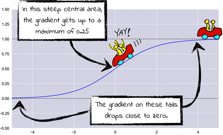
The sigmoid’s gradient reaches its maximum, that happens to be 0.25, right in the center. As you move along its tails, the gradient drops quickly. If the sigmoid receives a large input, either positive or negative, it enters a vicious circle:
- The larger the sigmoid’s input, the smaller the gradient.
- The smaller the gradient, the slower GD.
- The slower GD, the less the network’s weights change.
- The less the weights change, the less likely it is the sigmoid’s input will eventually shift back toward zero.
When the sigmoid enters this loop, the nodes uphill of the sigmoid become “dead neurons”. GD is unable to update them, and they stop learning. With too many dead neurons, the whole backprop process slows to a crawl.
This problem is compound by another subtle issue: the sigmoid is “off-center.” When it receives a value that’s close to zero, it shifts that value close to 0.5. We said that numbers close to zero are generally better, so it would be nice if the sigmoid didn’t go out of its way to push the numbers in the neural network far away from zero.
To wrap up, the sigmoid only works well when the values in the network are close to zero. That’s a though call, especially when the sigmoid itself tends to push values farther from zero. As they get farther from zero, those values slow down backpropagation and kill off the network’s neurons. The deeper the network, the more sigmoids it contains—and the worse this problem becomes.
Those issues have been known since people became using sigmoids in neural networks. In a deep network, however, they contribute to a worse problem—one that stumped machine learning researchers for years.
The Vanishing Gradient
Here’s our periodic reminder of how backpropagation works: It accumulates the local gradients of all the components in the network from the output to the input layer—like this:
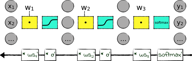
Backpropagation starts from the local gradient of the softmax in the output layer. Then it multiplies it by the gradient of the last weighted sum (that I called ![]() ’); it multiplies the result by the gradient of the last sigmoid… and so on, all the way back to the first layer. The gradient of the first layer is the product of the accumulated local gradients.
’); it multiplies the result by the gradient of the last sigmoid… and so on, all the way back to the first layer. The gradient of the first layer is the product of the accumulated local gradients.
Now, as you saw in the previous section, the local gradient of a sigmoid is a small number between 0 and 0.25. Whenever backprop traverses a sigmoid, the global gradient is multiplied by that small number, making it smaller. If the network has many layers—and many sigmoids—then the first layers in the network receive a minuscule gradient, and their weights barely change at all.
What I just described is the problem of the vanishing gradient. As it moves back through the network, the gradient becomes vanishingly small. This problem puts us in a catch-22: If we want a more powerful network, we should add layers to it; but the more layers we add, the smaller the gradients of the first layers become, to the point where those layers stop learning. We’re damned if we add layers, and damned if we don’t.
To wrap it all up, we uncovered two significant issues with the sigmoid:
-
The problem of dead neurons: with a large input, the sigmoid’s gradient tends toward zero.
-
The problem of vanishing gradients: each sigmoid diminishes the total gradient of the network to the point where the first layers receive a gradient that’s close to zero.
Both problems result in tiny gradients that slow down backpropagation, and maybe halt it for good.
Thank you for staying with me! It took us some time to go through this examination of the sigmoid. On a positive note, that’s nothing compared to the time it took researchers to identify some of these problems. For years they struggled to pinpoint why deep neural networks were so hard to train. Once they understood the problems, however, those researchers also came up with solutions. Let’s take a look at them.