Quantitative Analysis: From k-ratio to Composition

19.1 What Is a k-ratio?

A k-ratio is the ratio of a pair of characteristic X-ray line intensities, I, measured under similar experimental conditions for the unknown (unk) and standard (std):

$k={I}_{unk}/{I}_{\mathrm{std}}$

(19.1)

The measured intensities can be associated with a single characteristic X-ray line (as is typically the case for wavelength spectrometers) or associated with a family of characteristic X-ray lines (as is typically the case for energy dispersive spectrometers.) The numerator of the k-ratio is typically the intensity measured from an unknown sample and the denominator is typically the intensity measured from a standard material—a material of known composition.

Both the numerator and the denominator of the k-ratio must be measured under similar, well-controlled instrument conditions. The electron beam energy must be the same. The probe dose, the number of electrons striking the sample during the measurement, should be the same (or the intensity scaled to equivalent dose.) The position of the sample relative to the beam and to the detector should be fixed. Both the sample and the standard(s) should be prepared to a high degree of surface polish, ideally to reduce surface relief below 50 nm, and the surface should not be chemically etched. If the unknown is non-conducting, the same thickness of conducting coating, usually carbon with a thickness below 10 nm, should be applied to both the unknown and the standard(s). Ideally, the only aspect that should differ between the measurement of the unknown and the standard are the compositions of the materials.

The k-ratio is the first estimate of material composition. From a set of k-ratios, we can estimate the unknown material composition. In many cases, to a good approximation:

${C}_{Z,\mathrm{unk}}\sim {k}_Z{C}_{Z,\mathrm{std}}={I}_{\mathrm{unk}}/{I}_{\mathrm{std}}{C}_{Z,\mathrm{std}}$

(19.2)

where C _Z,unk and C _Z,std are the mass fraction of element Z in the unknown and standard, respectively, and k _Z is the k-ratio measured for element Z. This relationship is called “Castaing’s first approximation” after the seminal figure in X-ray microanalysis, who established the k-ratio as the basis for quantitative analysis (Castaing 1951).

By taking a ratio of intensities collected under similar conditions, the k-ratio is independent of various pieces of poorly known information.

1.
The k-ratio eliminates the need to know the efficiency of the detector since both sample and unknown are measured on the same detector at the same relative position. Since the efficiency as a multiplier of the intensity is identical in the numerator and denominator of the k-ratio, the efficiency cancels quantitatively in the ratio.
2.
The k-ratio mitigates the need to know the physics of the X-ray generation process if the same elements are excited under essentially the same conditions. The ionization cross section, the relaxation rates, and other poorly known physical parameters are the same for an element in the standard and the unknown.

In the history of the development of quantitative electron-excited X-ray microanalysis, the X-ray intensities for the unknown and standards were measured sequentially with a wavelength spectrometer in terms of X-ray counts. The raw measurement contains counts that can be attributed to both the continuum background (bremsstrahlung) and characteristic X-rays. Since k-ratio is a function of only the characteristic X-rays, the contribution of the continuum must be estimated. Usually, this is accomplished by measuring two off-peak measurements bounding the peak and using interpolation to estimate the intensity of the continuum background at the peak position. The estimated continuum is subtracted from the measured on peak intensity to give the characteristic X-ray line intensity.

Extracting the k-ratio with an energy dispersive spectrometer can be done in a similar manner for isolated peaks. However, to deal with the peak interferences frequently encountered in EDS spectra, it is necessary to simultaneously consider all of the spectrum channels that span the mutually interfering peaks. Through a process called linear least squares fitting, a scale factor is computed which represents the multiplicative factor by which the integrated area under the characteristic peak from the standard must be multiplied by to equal the integrated area under the characteristic peak from the unknown. This scale factor is the k-ratio, and the fitting process separates the intensity components of the interfering peaks and the continuum background. The integrated counts measured for the unknown and for the standard for element Z enable an estimate of the precision of the measurement for that element. Linear least squares fitting is employed in NIST DTSA-II to recover characteristic X-ray intensities, even in situations with extreme peak overlaps.

A measured k-ratio of zero suggests that there is none of the associated element in the unknown. A measurement on a standard with exactly the same composition as the unknown will nominally produce a k-ratio of unity for all elements present. Typically, k-ratios will fall in a range from 0 to 10 depending on the relative concentration of element Z in the unknown and the standard. A k-ratio less than zero can occur when count statistics and the fitting estimate of the background intensity conspire to produce a slightly negative characteristic intensity. Of course, there is no such thing as negative X-ray counts, and negative k-ratios should be set to zero before the matrix correction is applied. A k-ratio larger than unity happens when the standard generates fewer X-rays than the unknown. This can happen if the standard contains less of the element and/or if the X-ray is strongly absorbed by the standard. Usually, a well-designed measurement strategy won’t result in a k-ratio much larger than unity. We desire to use a standard where the concentration of element Z is high so as to minimize the contribution of the uncertainty in the amount of Z in the standard to the overall uncertainty budget of the measurement, as well as to minimize the uncertainty contribution of the count statistics in the standard spectrum to the overall measurement precision. The ideal standard to maximize concentration is a pure element, but for those elements whose physical and chemical properties prohibit them from being used in the pure state, for example, gaseous elements such as Cl, F, I, low melting elements such as Ga or In, or pure elements which deteriorate under electron bombardment, for example, P, S, a binary compound can be used, for example, GaP, FeS₂, CuS, KCl, etc.

TIP

To get the most accurate trace and minor constituent measurements, it is best to average together many k-ratios from distinct measurements before applying the matrix correction. Don’t truncate negative k-ratios before you average or you’ll bias your results in the positive direction.

19.2 Uncertainties in k-ratios

All k-ratio measurements must have associated uncertainty estimates. The primary source of uncertainty in a k-ratio measurement is typically count statistics although instrumental instability also can contribute. X-ray emission is a classic example of a Poisson process or a random process described by a negative exponential distribution.

Negative exponential distributions are interesting because they are “memoryless.” For a sequence of events described by a negative exponential distribution, the likelihood of an event’s occurring in an interval τ is equally as likely regardless of when the previous event occurred. Just because an event hasn’t occurred for a long time doesn’t make an event any more likely in the subsequent time interval. In fact, the most probable time for the next event is immediately following the previous.

If X-rays are measured at an average rate R, the average number of X-rays that will be measured over a time t is N = R · t. Since the X-ray events occur randomly dispersed in time, the actual number measured in a time t will rarely ever be exactly N = R · t. Instead, 68.2 % of the time the actual number measured will fall within the interval (N – ΔN, N + ΔN) where ΔN ~ N ^1/2 when N is large (usually true for X-ray counts). This interval is often called the “one sigma” interval. The one-sigma fractional uncertainty is thus N/N ^1/2 = 1/N ^1/2, which for constant R decreases as t increased. This is to say that generally, it is possible to make more precise measurements by spending more time making the measurement. All else remaining constant, for example, instrument stability and specimen stability under electron bombardment, a measurement taken for a duration of 4 t will have twice the precision of a measurement take for t.

Poisson statistics apply to both the WDS and EDS measurement processes. For WDS, the on-peak and background measurements all have associated Poissonian statistical uncertainties. For EDS, each channel in the spectrum has an associated Poissonian statistical uncertainty. In both cases, the statistical uncertainties must be taken into account carefully so that an estimate of the measurement precision can be associated with the k-ratio.

The best practices for calculating and reporting measurement uncertainties are described in the ISO Guide to Uncertainty in Measurement (ISO 2008). Marinenko and Leigh (2010) applied the ISO GUM to the problem of k-ratios and quantitative corrections in X-ray microanalytical measurements. In the case of WDS measurements, the application of ISO GUM is relatively straightforward and the details are in Marinenko and Leigh (2010). For EDS measurements, the process is more complicated. If uncertainties are associated with each channel in the standard and unknown spectra, the k-ratio uncertainties are obtained as part of the process of weighted linear squares fitting.

19.3 Sets of k-ratios

Typically, a single compositional measurement consists of the measurement of a number of k-ratios—typically one or more per element in the unknown. The k-ratios in the set are usually all collected under the same measurement conditions but need not be. It is possible to collect individual k-ratios at different beam energies, probe doses or even on different detectors (e.g., multiple wavelength dispersive spectrometers or multiple EDS with different isolation windows).

There may more than one k-ratio per element. Particularly when the data is collected on an energy dispersive spectrometer, more than one distinct characteristic peak per element may be present. For period 4 transition metals, the K and L line families are usually both present. In higher Z elements, both the L and M families may be present. This redundancy provides a question – Which k-ratio should be used in the composition calculation?

While it is in theory possible to use all the redundant information simultaneously to determine the composition, standard practice is to select the k-ratio which is likely to produce the most accurate measurement. The selection is non-trivial as it involves difficult to characterize aspects of the measurement and correction procedures. Historically, selecting the optimal X-ray peak has been something of an art. There are rules-of-thumb, but they involve subtle compromises and deep intuition.

This subject is discussed in more detail in Appendix 19.A. For the moment, we will assume that one k-ratio has been selected for each measured element.

$k=\left\{\ {k}_Z:Z\in elements\ \right\}$

(19.3)

Our task then becomes converting this set of k-ratios into an estimate of the unknown material’s composition.

$C=\left\{\ {C}_Z:Z\in elements\ \right\}$

(19.4)

19.4 Converting Sets of k-ratios Into Composition

As stated earlier, the k-ratio is often a good first approximation to the composition. However, we can do better. The physics of the generation and absorption of X-rays is sufficiently well understood that we can use physical models to compensate for non-ideal characteristics of the measurement process. These corrections are called matrix corrections as they compensate for differences in the matrix (read matrix to mean “material”) between the standard material and the unknown material.

Matrix correction procedures are typically divided into two classes φ(ρz) and ZAF-type corrections. The details will be discussed in Appendix 19.A. The distinction is primarily how the calculation is divided into independent sub-calculations. In a ZAF-type algorithm, the corrections for differences in mean atomic number (the Z term), X-ray absorption (the A term) and secondary fluorescence (the F term) are calculated separately. φ(ρz) matrix correction algorithms combine the Z and A terms into a single calculation. The distinction between φ(ρz) and ZAF is irrelevant for this discussion so the matrix correction will be described by the generic ZAF(C _A; P) where this expression refers to the matrix correction associated with a material with composition C_A and measurement parameters P. The terms k _Z and C _Z refer to the k-ratio and composition of the Z-th element in the unknown.

${k}_z=\frac{\mathrm{ZAF}\left({C}_{\mathrm{unk}};P\right)}{\mathrm{ZAF}\left({C}_{\mathrm{std}};P\right)}\frac{C_{\mathrm{unk}}}{C_{\mathrm{std}}}$

(19.5a)

To state the task clearly, we have measured {k _Z : Z ∈ elements}. We want to know which {C _Z : Z ∈ elements} produces the observed set of k-ratios.

${C}_{\mathrm{unk}}={k}_z\ {C}_{\mathrm{std}}\frac{ZAF\left({C}_{\mathrm{std}};P\right)}{ZAF\left({C}_{\mathrm{unk}};P\right)}$

(19.5b)

However, there is a problem. Our ability to calculate k _Z depends upon knowledge of the composition of the unknown, C _unk. Unfortunately, we don’t know the composition of the unknown. That is what we are trying to measure.

Fortunately, we can use a trick called “iteration” or successive approximation to solve this dilemma. The strategy is as follows:

1.
Estimate the composition of the unknown. Castaing’s First Approximation is a good place to start.
2.
Calculate an improved estimate of C_Z,unk based on the previous estimated composition.
3.
Update the composition estimate based on the new calculation.
4.
Test whether the resulting computed k-ratios are sufficiently similar to the measured k-ratios.
5.
Repeat steps 2–5 until step 4 is satisfied.

While there is no theoretical guarantee that this algorithm will always converge or that the result is unique, in practice, this algorithm has proven to be extremely robust.

19.5 The Analytical Total

The result of the iteration procedure is a set of estimates of the mass fraction for each element in the unknown. We know these mass fractions should sum to unity—they account for all the matter in the material. However, the measurement process is not perfect and even with the best measurements there is variation around unity.

The sum of the mass fractions is called the analytical total. The analytical total is an important tool to validate the measurement process. If the analytic total varies significantly from unity, it suggests a problem with the measurement. Analytical totals less than one can suggest a missed element (such as an unanticipated oxidized region of the specimen), a reduced excitation volume, an unanticipated sample geometry (film or inclusion), or deviation from the measurement conditions between the unknown and standard(s). Analytic totals greater than unity likely arise because of measurement condition deviation or sample geometry issues.

19.6 Normalization

As mentioned in the previous section, the analytical total is rarely exactly unity. When it isn’t, the accuracy of a measurement can often be improved by normalizing the measured mass fractions, C _i, by the analytical total of all N constituents to produce the normalized mass fractions, C _i,n:

${C}_{i,n}={C}_i/\underset{1}{\overset{N}{\varSigma }}{C}_i$

(19.6)

This procedure should be performed with care and the analytic total reported along with the normalized mass fractions. Normalization is not guaranteed to improve results and can cover up for some measurement errors like missing an element or inappropriately accounting for sample morphology. The analytical total is important information and the normalized mass fractions should never be reported without also reporting the analytical total. Any analysis which sums exactly to unity should be viewed with some skepticism.

Careful inspection of the raw analytical total is a critical step in the analytical process. If all constituents present are measured with a standards-based/matrix correction procedure, including oxygen (or another element) determined by the method of assumed stoichiometry, then the analytical total can be expected to fall in the range 0.98 to 1.02 (98 weight percent to 102 weight percent). Deviations outside this range should raise the analyst’s concern. The reasons for such deviations above and below this range may include unexpected changes in the measurement conditions, such as variations in the beam current, or problems with the specimen, such as local topography such as a pit or other excursion from an ideal flat polished surface. For a deviation below the expected range, an important additional possibility is that there is at least one unmeasured constituent. For example, if a local region of oxidation is encountered while analyzing a metallic sample, the analytical total will drop to approximately 0.7 (70 weight percent) because of the significant fraction of oxygen in a metal oxide. Note that “standardless analysis” (see below) may automatically force the analytical total to unity (100 weight percent) because of the loss of knowledge of the local electron dose used in the measurement. Some vendor software uses a locally measured spectrum on a known material, e.g., Cu, to transfer the local measurement conditions to the conditions used to measure the vendor spectrum database. Another approach is to use the peak-to-background to provide an internal normalization. Even with these approaches, the analytical total may not have as narrow a range as standards-based analysis. The analyst must be aware of what normalization scheme may be applied to the results. An analytical total of exactly unity (100 weight percent) should be regarded with suspicion.

19.7 Other Ways to Estimate C_Z

k-ratios are not the only information we can use to estimate the amount of an element Z, C _Z. Sometimes it is not possible or not desirable to measure k _Z. For example, low Z elements, like H or He, don’t produce X-rays or low Z elements like Li, B and Be produce X-rays which are so strongly absorbed that few escape to be measured. In other cases, we might know the composition of the matrix material and all we really care about is a trace contaminant. Alternatively, we might know that certain elements like O often combine with other elements following predictable stoichiometric relationships. In these cases, it may be better to inject other sources of information into our composition calculation algorithm.

19.7.1 Oxygen by Assumed Stoichiometry

Oxygen can be difficult to measure directly because of its relatively low energy X-rays. O X-rays are readily absorbed by other elements. Fortunately, many elements combine readily with oxygen in predictable ratios. For example, Si oxidizes to form SiO₂ and Al oxidizes to form Al₂O₃. Rather than measure O directly, it is useful to compute the quantity of other elements from their k-ratios and then compute the amount of O it would take to fully oxidize these elements. This quantity of O is added in to the next estimated composition.

NIST DTSA-II has a table of common elemental stoichiometries for calculations that invoke assumed stoichiometry. For many elements, there may be more than one stable oxidation state. For example, iron oxidizes to FeO (wüstite), Fe₃O₄ (magnetite), and Fe₂O₃ (hematite). All three forms occur in natural minerals. The choice of oxidation state can be selected by the user, often relying upon independent information such as a crystallographic determination or based upon the most common oxidation state that is encountered in nature.

The same basic concept can be applied to other elements which combine in predicable ratios.

19.7.2 Waters of Crystallization

Water of crystallization (also known as water of hydration or crystallization water) is water that occurs within crystals. Typically, water of crystallization is annotated by adding “·nH₂O” to the end of the base chemical formula. For example, CuSO₄ · 5H₂O is copper(II) sulfate pentahydrate. This expression indicates that five molecules of water have been added to copper sulfate. Crystals may be fully hydrated or partially hydrated depending upon whether the maximum achievable number of water molecules are associated with each base molecule. CuSO₄ is partially hydrated if there are fewer than five water molecules per CuSO₄ molecule. Some crystals hydrate in a humid environment. Hydration molecules (water) can often be driven off by strong heating, and some hydrated materials undergo loss of water molecules due to electron beam damage.

Measuring water of crystallization involves measuring O directly and comparing this measurement with the amount of water predicted by performing a stoichiometric calculation on the base molecule. Any surplus oxygen (oxygen measured but not accounted for by stoichiometry) is assumed to be in the form of water and two additional hydrogen atoms are added to each surplus oxygen atom. The resulting composition can be reported as the base molecule + “·nH₂O” where n is the relative number waters per base molecule.

19.7.3 Element by Difference

All matter consists of 100 % of some set of elements. If we were able to measure the mass fraction of N-1 of the N elements in a material with perfect accuracy then the mass fraction of the Nth element would be the difference

${C}_N=1-\sum \limits_{i=1}^{N-1}{C}_i$

(19.7)

Of course, we can’t measure the N-1 elements with perfect accuracy, but we can apply the same concept to estimate the quantity of difficult to measure elements.

This approach has numerous pitfalls. First, the uncertainty in difference is the sum of the uncertainties for the mass fractions of the N-1 elements. This can be quite large particularly when N is large. Second, since we assume the total mass fraction sums to unity, there is no redundant check like the analytic total to validate the measurement.

19.8 Ways of Reporting Composition

19.8.1 Mass Fraction

The most common way to report the composition of a material is in terms of the mass fraction. To understand the mass fraction, consider a block of material containing a mixture of different atoms. Weigh the block. Now imagine separating the block into distinct piles, each pile containing all the atoms from one element in the block. Weigh each of the separated piles. The mass fraction is calculated as the ratio of the mass of pile containing element Z over the total mass of the block. Since each element in the block is represented by a pile and since none of the atoms are lost in the process of dividing the block, the sum of mass fractions equals unity. Of course, we can’t really do this measurement this way for most materials but conceptually we can understand mass fraction as though we can. As a simple example, consider the mineral pyrite, FeS₂. The molecular formula combines one gram-mole of Fe (atomic weight A = 55.85 g/mole) with two gram moles of S (A = 32.07 g/mole) for a compound molecular weight of 119.99 g/mole. The mass fractions, C _w, of the constituents are thus

${C}_{w, Fe}=55.85/119.99=0.4655$

(19.8a)

${C}_{w,S}=64.14/119.99=0.5345$

(19.8b)

The mass fraction is the fundamental output of electron probe X-ray microanalysis measurements. All other output modes are calculated from the mass fraction.

Weight fraction, mass percent, weight percent are all commonly seen synonyms for mass fractions. Mass fraction or mass percent is the preferred nomenclature because it is independent of local gravity.

19.8.2 Atomic Fraction

If we perform the same mental experiment as was described in the mass fraction section, but instead of weighing the piles, we instead count the number of atoms in the block and each of the piles. If we then calculate the ratio of the number of atoms of element Z relative to the total number of atoms in the block, this is the atomic fraction, C _a. For the example of FeS₂, which contains a total of three atoms in the molecular formula, the atomic fractions are

${C}_{a, Fe}=1/3=0.3333$

(19.9a)

${C}_{a,S}=2/3=0.6667$

(19.9b)

We can calculate atomic fraction C _a from mass fraction C _w and vice versa using the atomic weights A of the elements.

${C}_{a,i}=\left({C}_{w,i}/{A}_i\right)/\underset{1}{\overset{N}{\varSigma }}\left({C}_{w,i}/{A}_i\right)$

(19.10)

Where N is the number of elements involved in the mixture.

Starting with the atomic fractions, the mass fractions are calculated according to the formula

${C}_{w,i}=\left({C}_{a,i}\ast {A}_i\right)/\underset{1}{\overset{N}{\varSigma }}\left({C}_{a,i}\ast {A}_i\right)$

(19.11)

It is appropriate to use the atomic weights as suggested by the IUPAC (► http://www.ciaaw.org/atomic_weights4.htm). These weights are based on assumed mixes of isotopes as are typically seen in terrestrial samples. Occasionally, when it is known that an element is present in a perturbed isotopic mix, it may be appropriate to use this information to calculate a more accurate atomic weight. Since the atomic fraction depends upon assumed atomic weights, the atomic fraction is less fundamental than the mass fraction.

19.8.3 Stoichiometry

Stoichiometry is closely related to atomic fraction. Many materials can be described simply in terms of the chemical formula of its most basic constituent unit. For example, silicon and oxygen combine to form a material in which the most basic repeating element consists of SiO₂. Stoichiometry can be readily translated into atomic fraction. Since our measurements are imprecise, the stoichiometry rarely works out in clean integral units. However, the measurement is often precise enough to distinguish between two or more valence states.

19.8.4 Oxide Fractions

Oxide fractions are closely related to stoichiometry. When a material such as a natural mineral is a mixture of oxides, it can make sense to report the composition as a linear sum of the oxide constituents by mass fraction.

◘ Table 19.1 shows the analysis of NIST SRM470 (K412 glass) with the results reported as oxide fraction, mass fraction, and atomic fraction.

Table 19.1

Three different ways to report the composition of NIST SRM 470 glass K412.

K412 Glass
Element	Mg	Al	Si	Ca	Fe	O	Sum
Valence	2	3	1	2	2	−2	–
Atomic weight (AMU)	24.305	26.9815	28.085	40.078	55.845	15.999
Oxide fraction	0.1933 ± 0.0020 MgO	0.0927 ± 0.0020 Al₂O₃	0.4535 ± 0.0020 Si0₂	0.1525 ± 0.0020 CaO	0.0996 ± 0.0020 FeO	–	0.9916
Mass fraction	0.1166	0.0491	0 2120	0.1090	0.0774	0 4276	0.9916
Atomic fraction	0.1066	0.0404	0.1678	0.0604	0.0308	0.5940	1

19.8.4.1 Example Calculations

Calculating the mass fraction from the oxide fraction for Al in K412 glass:

${C}_{w, Al}=\frac{2\times 26.9815}{2\times 26.9815+3\times 15.999}0.0927=0.04906$

(19.12)

Calculating the atomic fraction from the mass fraction:

${C}_{a, Al}=\frac{\frac{0.0491}{26.9815}}{\frac{0.1166}{24.305}+\frac{0.0491}{26.9815}+\frac{0.2120}{28.085}+\frac{0.1090}{40.078}+\frac{0.0774}{55.845}+\frac{0.4275}{15.999}}$

(19.13)

19.9 The Accuracy of Quantitative Electron-Excited X-ray Microanalysis

19.9.1 Standards-Based k-ratio Protocol

Quantitative electron-excited X-ray microanalysis following the standards-based k-ratio protocol is a relative not an absolute analysis method. The unknown is measured relative to standards of well known composition such as pure elements and stoichiometric compounds with fixed atom ratios, for example, FeS₂. The accuracy of the method can only be tested by analyzing materials whose composition is known from independent (and ideally absolute) analysis methods and whose composition has been found to be homogeneous at the sub-micrometer scale. There are limited numbers of special materials that fit these strict compositional requirements to qualify as certified reference materials for electron beam X-ray microanalysis, including certain metal alloys, intermetallic compounds, and glasses. Limited numbers of these materials are available from national standards institutions, such as the National Institute of Standards and Technology (U.S.) (e.g., Marinenko et al. 1990) and the European Commission Community Bureau of Reference (e.g., Saunders et al. 2004). Certain mineral species have been characterized to serve as standards, which are of particular use to the geochemistry community, by the Smithsonian Institution. These certified reference materials and related materials such as minerals can serve directly as standards for analyses, but their other important function is to serve as challenge materials to test the quantification methods. Additional materials suitable for testing the method include stoichiometric compounds with formulae that define specific, unvarying compositions; that is, the same materials that can also be used as standards. Thus, FeS₂ could be used as an “unknown” for a test analysis with Fe and CuS as the standards, while CuS could be analyzed with Cu and FeS₂ as standards. From such analyses of certified reference materials and other test materials, the relative deviation from the expected value (RDEV) (also referred to as “relative error”) is calculated with the “expected” value taken as the stoichiometric formula value or the value obtained from an “absolute” analytical method, such as gravimetric analysis:

$\mathrm{RDEV}=\left[\frac{\left(\mathrm{Analyzed}\ \mathrm{value}-\mathrm{expected}\ \mathrm{value}\right)}{\mathrm{expected}\ \mathrm{value}}\right]\times 100\%$

(19.14)

Note that by this equation a positive RDEV indicates an overestimate of the concentration, while a negative RDEV indicates an underestimate. By analyzing many test materials spanning the periodic table and determining the relative deviation from the expected value (relative error), the analytical performance can be estimated. For example, early studies of quantitative electron probe microanalysis with wavelength dispersive X-ray spectrometry following the standards-based k-ratio protocol and ZAF matrix corrections produced a distribution of RDEV values (relative errors) such that 95 % of the analyses were captured in an RDEV (relative error) range of ±5 % relative, as shown in ◘ Fig. 19.1 (Yakowitz 1975).

../images/271173_4_En_19_Chapter/271173_4_En_19_Fig1_HTML.png — Fig. 19.1
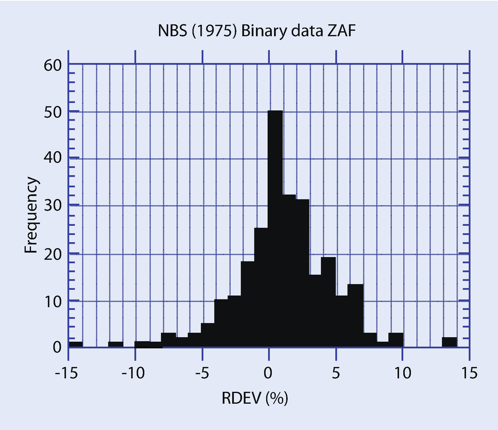
Histogram of relative deviation from expected value (relative error) for electron probe microanalysis with wavelength dispersive spectrometry following the k-ratio protocol with standards and ZAF corrections (Yakowitz 1975)

Subsequent development and refinement of the matrix correction procedures by many researchers improved upon this level of accuracy. Pouchou and Pichoir (1991) described an advanced matrix correction model based upon extensive experimental measurements of the φ(ρz) description of the depth distribution of ionization. Incorporating explicit measurements for low energy photons, this approach has been especially successful for low photon energy X-rays which were subject to high absorption. A comparison of corrections of the same k-ratio dataset with their φ(ρz) method and with the conventional ZAF method showed significant narrowing of the RDEV distribution and elimination of significant large RDEV values, as shown in ◘ Fig. 19.2. With this improvement, approximately 95 % of analyses fall within ±2.5 % RDEV.

../images/271173_4_En_19_Chapter/271173_4_En_19_Fig2_HTML.png — Fig. 19.2
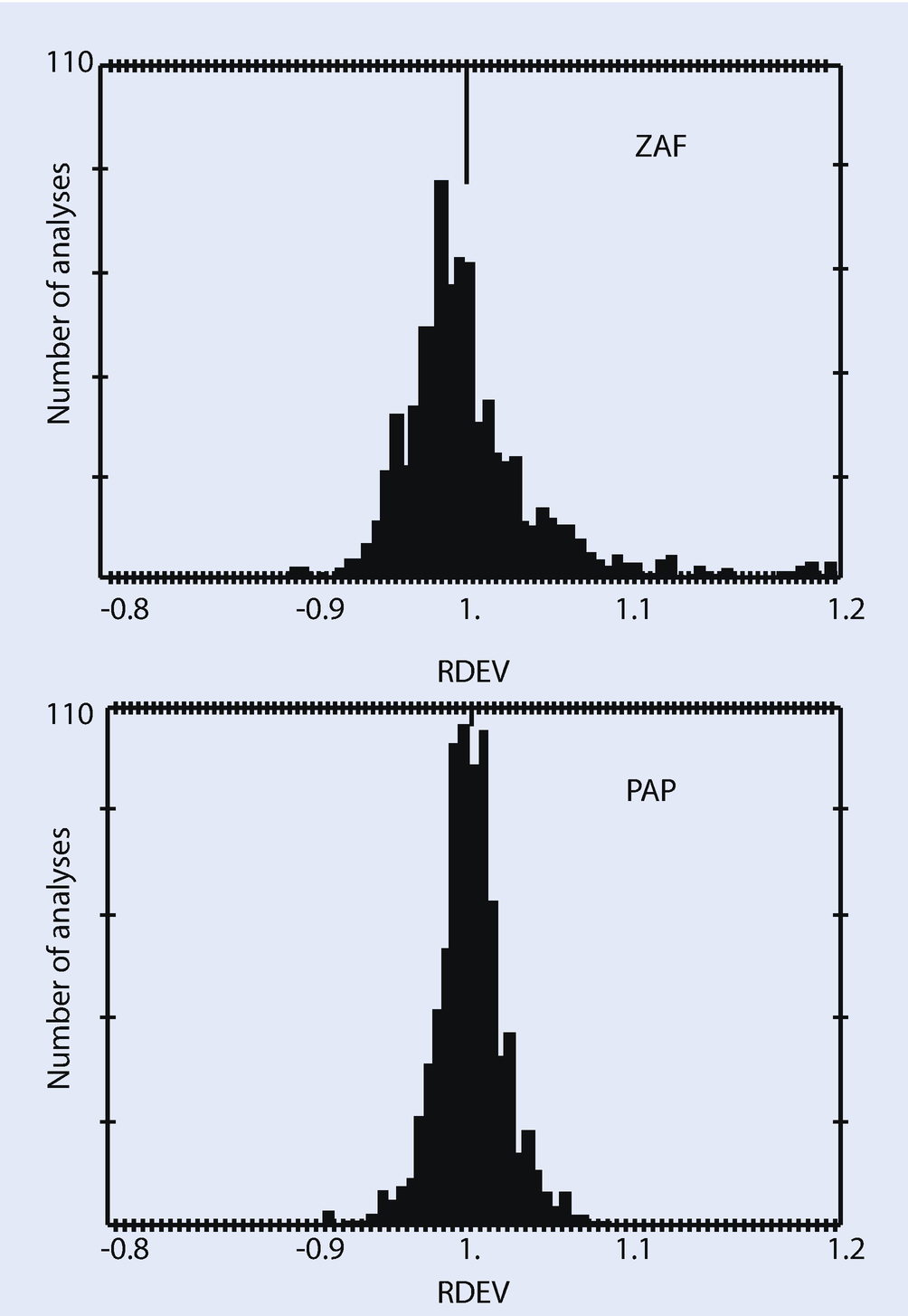
Comparison of quantitative analysis of an EPMA-WDS k = ratio database by conventional ZAF and by the PAP φ(ρz) model (Pouchou and Pichoir 1991)

► Chapter 20 will illustrate examples of quantitative electron-excited X-ray microanalysis with silicon drift detector (SDD)-EDS performed on flat bulk specimens following the k-ratio protocol and PAP φ(ρz) matrix corrections with NIST DTSA-II. The level of accuracy achieved with this SDD-EDS approach fits within the RDEV histogram achieved with EPMA-WDS for major, minor, and trace constituents, even when severe peak interference occurs. It should be noted that SDD-EDS is sufficiently stable with time that, providing a quality measurement protocol is in place to ensure that all measurements are made under identical conditions of beam energy, known dose, specimen orientation, and SDD-EDS performance, archived standards can be used without significant loss of accuracy.

19.9.2 “Standardless Analysis”

Virtually all vendor analytical software includes the option for “standardless analysis.” Standardless analysis requires only the spectrum of the unknown, the list of elements identified during qualitative analysis, and the beam energy; and the software will report quantitative concentration values, including oxygen by assumed stoichiometry if desired. “Standardless analysis” is usually implemented as a “black box” tool without extensive documentation. The approach is the same as the standards-based analysis protocol: a k-ratio is the starting point, but the spectrum of the unknown only provides the numerator of the k-ratio. A “first principles physics” calculation of the standard intensity for the denominator of the k-ratio, while possible, is difficult because of the lack of accurate values of critical parameters in the equations for X-ray generation and propagation. Instead, the general approach employed throughout the EDS industry is the use of a library of remotely measured standards to provide the intensity for the denominator of the k-ratio. Pure element and binary compound standards are measured under defined conditions at several beam energies on a well characterized EDS. When standardless analysis is invoked, the appropriate elemental intensities are selected from this database of standards, and any missing elements not represented in the database are supplied by interpolation aided by the physical equations of X-ray generation and propagation. If a beam energy is requested for which reference values are not available in the database, the equations of the physics of X-ray generation are used to appropriately adjust the available intensities. Usually a reference spectrum that is locally measured on a pure element, for example, Mn or Cu, is used to compare the efficiency of the EDS on a channel-by-channel basis to the vendor EDS that was originally used to measure the standards library. Because of its simplicity of operation, standardless analysis enjoys great popularity. Probably 95 % or more of quantitative EDS analyses are performed with the standardless analysis procedure. While it is useful and is continually being improved, standardless analysis is subject to a substantially wider RDEV distribution than standards-based analysis with locally measured standards. Standardless analysis of a wide range of test materials produced the RDEV histogram shown in ◘ Fig. 19.3 (Newbury et al. 1995). This distribution is such that 95 % of all analyses fall within a range of ±25 % relative. If this level of analytical accuracy is sufficient, then standardless analysis is an acceptable procedure, providing this RDEV distribution, or a version appropriate to the standardless analysis software supplied by the vendor, is used to inform those who will make use of the quantitative analyses of the possible range of the results. While the standardless protocol may eventually equal the performance of standards-based analysis, recent results for current versions of standardless analysis, reported in ◘ Fig. 19.4, suggest that a wide RDEV distribution is still being experienced, at least from some vendors.

../images/271173_4_En_19_Chapter/271173_4_En_19_Fig3_HTML.png — Fig. 19.3
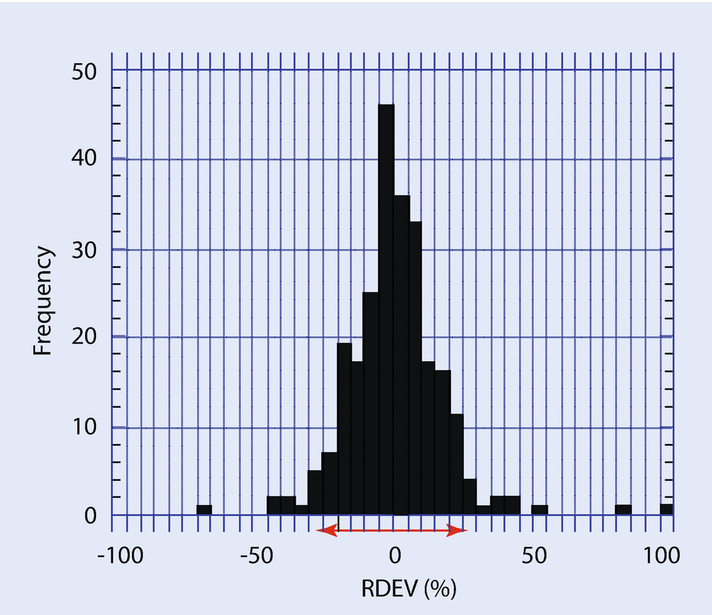
RDEV distribution observed for a vendor standardless analysis procedure (Newbury et al. 1995)

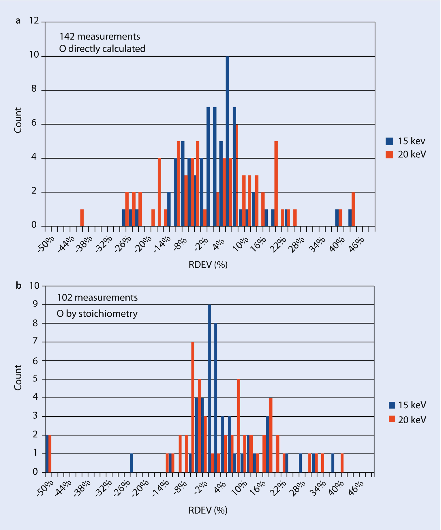
../images/271173_4_En_19_Chapter/271173_4_En_19_Fig4_HTML.png — Fig. 19.4
a RDEV distribution observed for a vendor standardless analysis procedures in 2016 with oxygen calculated directly for oxidized specimens. b RDEV distribution observed for a vendor standardless analysis procedures in 2016 with oxygen calculated by stoichiometry for oxidized specimens

It should be noted that when 95 % of all analyses fall within a range of ±25 % relative, it may often not be possible to correctly determine the formula of the major constituents of a stoichiometric compound. An example of this situation is presented in ◘ Table 19.2, which gives the results of an SEM-EDS analysis of a YBa₂Cu₃O_7-X single crystal by the k-ratio/standards protocol (NIST DTSA) compared to standardless analysis performed with two different vendors’ software. While the proper formula is recovered with the standards-based analysis, the formulae calculated from the standardless results do not match the proper formula.

Table 19.2

SEM-EDS analysis of a YBa₂Cu₃O_7-x single crystal (O calculated by stoichiometry)

	Y (true) 0.133 mass conc	Ba (true) 0.412	Cu (true) 0.286
k-ratio Stds ZAF	0.138 (+4 %)	0.411 (−0.2 %)	0.281 (−2 %) Cu-K Y₁Ba₂Cu₃O_6.4
Standards: Y and Cu pure elements; Ba (NIST glass K309)
Standardless Analysis (two different vendors):
M1	0.173 (+30 %)	0.400 (−3 %)	0.267 (−7 %) Cu-K Y₂Ba₃Cu₄O₁₀
M1	0.158 (+19 %)	0.362 (−12 %)	0.316 (+10 %) Cu-L Y₂Ba₃Cu₆O₁₂
M2	0.165 (+24 %)	0.387 (−6 %)	0.287 (+0.4 %) Cu-K Y₂Ba₃Cu₅O₁₁
M2	0.168 (+26 %)	0.395 (−4 %)	0.276 (−3.5 %) Cu-L Y₄Ba₆Cu₉O₂₁

Another shortcoming of standardless analysis is the loss of the information on the dose and the absolute spectrometer efficiency that is automatically embedded in the standards-based k-ratio/matrix corrections protocol. Without the dose and absolute spectrometer efficiency information, standardless analysis results must inevitably be internally normalized to unity (100 %) so that the calculated concentrations have realistic meaning, thereby losing the very useful information present in the raw analytical total that is available in the standards-based k-ratio/matrix corrections protocol. It must be noted that standardless analysis results will always sum to unity, even if one or more constituents are not recognized during qualitative analysis or are inadvertently lost from the suite of elements being analyzed. If the local dose and spectrometer efficiency can be accurately scaled to the conditions used to record remote standards, then standardless analysis can determine a meaningful analytical total, but this is not commonly implemented in vendor software.

19.10 Appendix

19.10.1 The Need for Matrix Corrections To Achieve Quantitative Analysis

There has long been confusion around the definition of the expression ‘ZAF’ used to compensate for material differences in X-ray microanalysis measurements. There are two competing definitions. Neither is wrong and both exist in the literature and implemented in microanalysis software. However, the two definitions lead to numerical values of the matrix corrections that are related by being numerical inverses of each other.

For the sake of argument, let’s call these two definitions ZAF _A and ZAF _B. In both definitions, $k={I}_{unk}/{I}_{std}$ and C _unk is the mass fraction of the element in the unknown.

ZAF _A is defined by the expression:

$k={C}_{unk} ZA{F}_A$

(19.15a)

ZAF _B is defined by the expression:

${C}_{unk}=k\ ZA{F}_B$

(19.15b)

If we solve each equation for k/C _unk and equate the resulting expression, we discover that

$ZA{F}_A=1/ ZA{F}_B$

(19.15c)

Needless to say, these inconsistent definitions can cause significant confusion. Whenever interpreting matrix corrections in the literature, it is important to identify which convention the author is using.

The confusion extends to this book. Most of this book has been written using the first convention (ZAF _A) however, the previous (third) edition of this book used the second convention (ZAF _B). The following section which has been pulled from the third edition continues to use the ZAF _B convention as this was the definition favored by the writer. NIST DTSA-II and CITZAF uses the $k={C}_{unk}\ ZA{F}_A$ convention.

(Contribution of the late Prof. Joseph Goldstein taken from SEMXM-3, ► Chapter 9)

Upon initial examination, it would seem that quantitative analysis should be extremely simple. Just form the ratio of the characteristic X-ray intensity for a given element measured from the specimen to that measured from the standard, and that ratio should be equal to the ratio of concentrations for a given element between the specimen and the standard. As was first noted by Castaing (1951), the primary generated intensities are roughly proportional to the respective mass fractions of the emitting element. If other contributions to X-ray generation are very small, the measured intensity ratios between specimen and standard are roughly equal to the ratios of the mass or weight fractions of the emitting element. This assumption is often applied to X-ray quantitation and is called Castaing’s “first approximation to quantitative analysis” and is given by

${C}_{\mathrm{i},\mathrm{unk}}/{C}_{i, std}={I}_{i, unk}/{I}_{i,\mathrm{std}}=k$

(19.16)

The terms C _i,unk and C _i,std are the composition in weight (mass) concentration of element i in the unknown and in the standard, respectively. The ratio of the measured unknown-to- standard intensities after continuum background is subtracted and peak overlaps are accounted for, I _i,unk/I _i,std, is the basic experimental measurement which underlies all quantitative X-ray microanalysis and is given the special designation as the “k-ratio.”

Careful measurements performed on homogeneous substances of known multi-element composition compared to pure element standards reveal that there are significant systematic deviations between the ratio of measured intensities and the ratio of concentrations. An example of these deviations is shown in ◘ Fig. 19.5, which depicts the deviations of measured X-ray intensities in the iron-nickel binary system from the linear behavior predicted by the first approximation to quantitative analysis, Eq. (19.16). ◘ Figure 19.5 shows the measurement of I _i,unk/I _i,std = k for Ni K-L₃ and Fe K-L₃ in nine well-characterized homogeneous Fe-Ni standards (Goldstein et al. 1965). The data were taken at an initial electron beam energy of 30 keV and a take-off angle ψ = 52.5°. The intensity ratio k _Ni or k _Fe is the I _i,unk/I _i,std measurement for Ni and Fe, respectively, relative to pure element standards. The straight lines plotted between pure Fe and pure Ni indicate the relationship between composition and intensity ratio given in Eq. (19.16). For Ni K-L₃, the actual data fall below the linear first approximation and indicate that there is an X-ray absorption effect taking place, that is, more absorption in the sample than in the standard. For Fe K-L₃, the measured data fall above the first approximation and indicate that there is a fluorescence effect taking place in the sample. In this alloy the Ni K-L₃ radiation is heavily absorbed by the iron and the Fe K-L₃ radiation is increased due to X-ray fluorescence by the Ni K-L₃ radiation over that generated by the bombarding electrons.

../images/271173_4_En_19_Chapter/271173_4_En_19_Fig5_HTML.png — Fig. 19.5
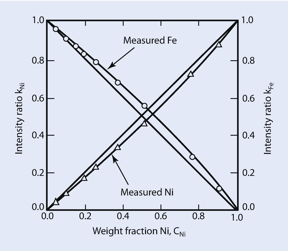
Measured Fe K-L₃ and Ni K-L₃ k-ratios versus the weight fraction of Ni at E ₀ = 30 keV. Curves are measured k-ratio data, while straight lines represent ideal behavior (i.e., no matrix effects)

These effects that cause deviations from the simple linear behavior given by Eq. (19.16) are referred to as matrix or inter-element effects. As described in the following sections, the measured intensities from specimen and standard need to be corrected for differences in electron backscatter and energy loss, X-ray absorption along the path through the solid to reach the detector, and secondary X-ray generation and emission that follows absorption, in order to arrive at the ratio of generated intensities and hence the value of C _i,unk. The magnitude of the matrix effects can be quite large, exceeding factors of ten or more in certain systems. Recognition of the complexity of the problem of the analysis of solid samples has led numerous investigators to develop the theoretical treatment of the quantitative analysis scheme, first proposed by Castaing (1951).

19.10.2 The Physical Origin of Matrix Effects

What is the origin of these matrix effects? The X-ray intensity generated for each element in the specimen is proportional to the concentration of that element, the probability of X-ray production (ionization cross section) for that element, the path length of the electrons in the specimen, and the fraction of incident electrons which remain in the specimen and are not backscattered. It is very difficult to calculate the absolute generated intensity for the elements present in a specimen directly. Moreover, the intensity that the analyst must deal with is the measured intensity. The measured intensity is even more difficult to calculate, particularly because absorption and fluorescence of the generated X-rays may occur in the specimen, thus further modifying the measured X-ray intensity from that predicted on the basis of the ionization cross section alone. Instrumental factors such as differing spectrometer efficiency as a function of X-ray energy must also be considered. Many of these factors are dependent on the atomic species involved. Thus, in mixtures of elements, matrix effects arise because of differences in elastic and inelastic scattering processes and in the propagation of X-rays through the specimen to reach the detector. For conceptual as well as calculational reasons, it is convenient to divide the matrix effects into atomic number, Z _i; X-ray absorption, A _i; and X-ray fluorescence, F _i, effects.

Using these matrix effects, the most common form of the correction equation is

${C}_{\mathrm{i},\mathrm{unk}}/{C}_{\mathrm{i},\mathrm{std}}=={\left[\mathrm{ZAF}\right]}_{\mathrm{i}}\left[{\mathrm{I}}_{\mathrm{i},\mathrm{unk}}/{\mathrm{I}}_{\mathrm{i},\mathrm{std}}\right]={\left[ ZAF\right]}_{\mathrm{i}}.{k}_{\mathrm{i}}$

(19.17)

where C _i,unk is the weight fraction of the element of interest in the unknown and C _i,std is the weight fraction of i in the standard. This equation must be applied separately for each element present in the sample. Equation (19.17) is used to express the matrix effects and is the common basis for X-ray microanalysis in the SEM/EPMA.

It is important for the analyst to develop a good idea of the origin and the importance of each of the three major non-linear effects on X-ray measurement for quantitative analysis of a large range of specimens.

19.10.3 ZAF Factors in Microanalysis

The matrix effects Z, A, and F all contribute to the correction for X-ray analysis as given in Eq. (19.17). This section discusses each of the matrix effects individually. The combined effect of ZAF determines the total matrix correction.

19.10.3.1 Atomic Number Effect, Z (Effect of Backscattering [R] and Energy Loss [S])

One approach to the atomic number effect is to consider directly the two different factors, backscattering (R) and stopping power (S), which determine the amount of generated X-ray intensity in an unknown. Dividing the stopping power, S, for the unknown and standard by the backscattering term, R, for the unknown and standard yields the atomic number matrix factor, Z _i, for each element, i, in the unknown. A discussion of the R and S factors follows.

Backscattering, R: The process of elastic scattering in a solid sample leads to backscattering which results in the premature loss of a significant fraction of the beam electrons from the target before all of the ionizing power of those electrons has been expended generating X-rays of the various elemental constituents. From ◘ Fig. 2.3a, which depicts the backscattering coefficient as a function of atomic number, this effect is seen to be strong, particularly if the elements involved in the unknown and standard have widely differing atomic numbers. For example, consider the analysis of a minor constituent, for example, 1 weight %, of aluminum in gold, against a pure aluminum standard. In the aluminum standard, the backscattering coefficient is about 15 % at a beam energy of 20 keV, while for gold the value is about 50 %. When aluminum is measured as a standard, about 85 % of the beam electrons completely expend their energy in the target, making the maximum amount of Al K-L₃ X-rays. In gold, only 50 % are stopped in the target, so by this effect, aluminum dispersed in gold is actually under represented in the X-rays generated in the specimen relative to the pure aluminum standard. The energy distribution of backscattered electrons further exacerbates this effect. Not only are more electrons backscattered from high atomic number targets, but as shown in ◘ Fig. 2.16a, b, the backscattered electrons from high atomic number targets carry off a higher fraction of their incident energy, further reducing the energy available for ionization of inner shells. The integrated effects of backscattering and the backscattered electron energy distribution form the basis of the “R-factor” in the atomic number correction of the “ZAF” formulation of matrix corrections.

Stopping power, S: The rate of energy loss due to inelastic scattering also depends strongly on the atomic number. For quantitative X-ray calculations, the concept of the stopping power, S, of the target is used. S is the rate of energy loss given by the Bethe continuous energy loss approximation, Eq. (1.1), divided by the density, ρ, giving S = − (1/ρ)(dE/ds). Using the Bethe formulation for the rate of energy loss (dE/ds), one observes that the stopping power is a decreasing function of atomic number. The low atomic number targets actually remove energy from the beam electron more rapidly with mass depth (ρz), the product of the density of the sample (ρ), and the depth dimension (z) than high atomic number targets.

An example of the importance of the atomic number effect is shown in ◘ Fig. 19.6. This figure shows the measurement of the intensity ratio k _Au and k _Cu for Au L-M and Cu K-L₃ for four well-characterized homogeneous Au-Cu standards (Heinrich et al. 1971). The data were taken at an initial electron beam energy of 15 keV and a take-off angle of 52.5°, and pure Au and pure Cu were used as standards. The atomic number difference between these two elements is 50. The straight lines plotted on ◘ Fig. 19.6 between pure Au and pure Cu indicate the relationship between composition and intensity ratio given in Eq. (19.17). For both Au L-M and Cu K-L₃, the absorption matrix effect, A _i, is less than 1 %, and the fluorescence matrix effect, F _i, is less than 2 %. For Cu K-L₃, the measured data fall above the first approximation and almost all the deviation is due to the atomic number effect, the difference in atomic number between the Au-Cu alloy and the Cu standard. As an example, for the 40.1 wt% Au specimen, the atomic number matrix factor, Z _Cu, is 1.12, an increase in the Cu K-L₃ intensity by 12 %. For Au L-M, the measured data fall below Castaing‘s first approximation and almost all the deviation is due to the atomic number effect. As an example, for the 40.1 wt % Au specimen, the atomic number effect, Z _Au, is 0.806, a decrease in the Au L-M intensity by 20 %. In this example, the S factor is larger and the R factor is smaller for the Cu K-L₃ X-rays leading to a larger S/R ratio and hence a larger Z _Cu effect. Just the opposite is true for the Au L-M X-rays leading to a smaller Z _Au effect. The effects of R and S tend to go in opposite directions and to cancel.

../images/271173_4_En_19_Chapter/271173_4_En_19_Fig6_HTML.png — Fig. 19.6
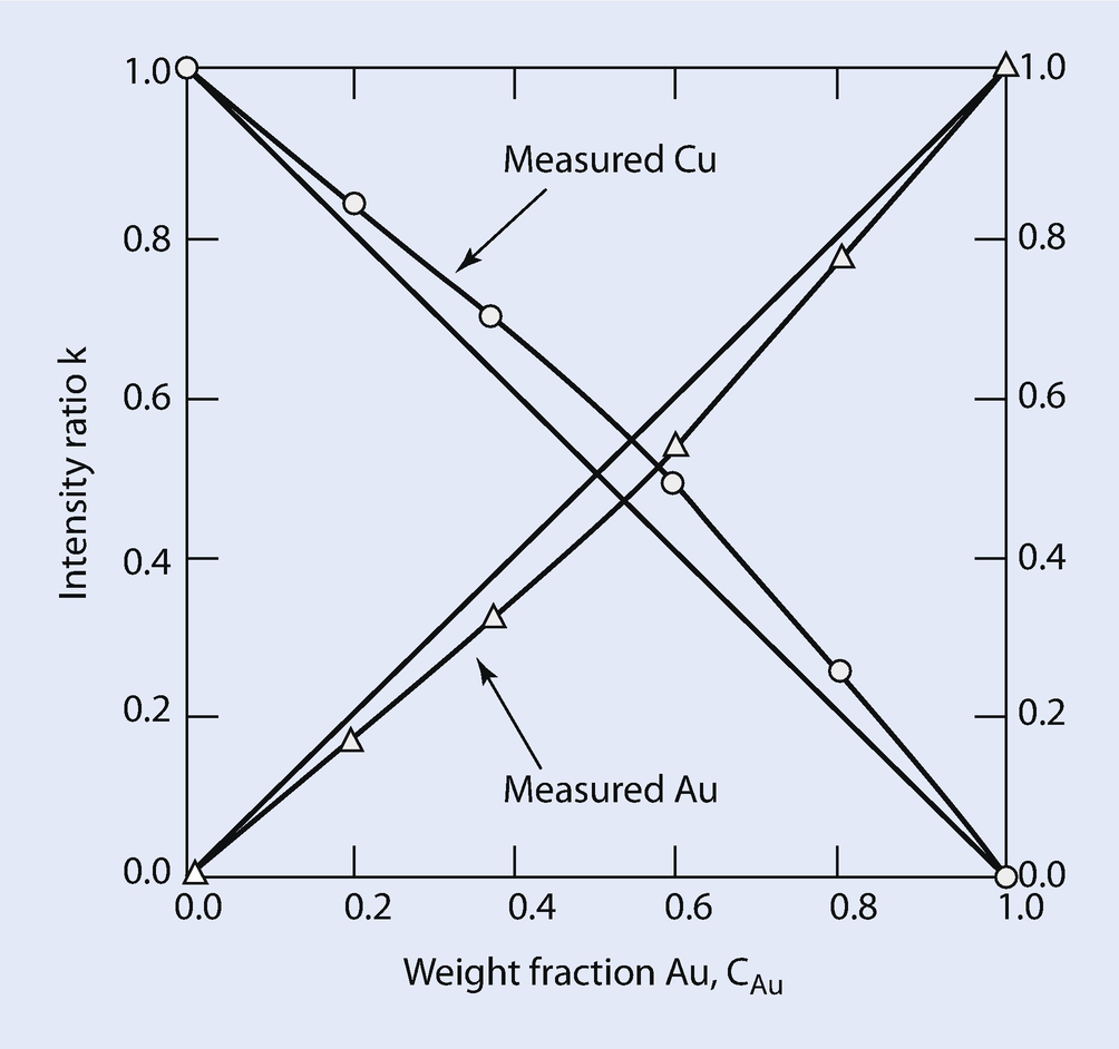
Measured Au L₃-M₅ and Cu K-L₃ k-ratios versus the weight fraction of Au at E ₀ = 25 keV. Curves are measured k-ratio data, while straight lines represent ideal behavior (i.e., no matrix effects)

X-ray Generation With Depth, φ(ρz)

A second approach to calculating the atomic number effect is to determine the X-ray generation in depth as a function of atomic number and electron beam energy. As shown in ► Chapters 1, 2, and 4, the paths of beam electrons within the specimen can be represented by Monte Carlo simulations of electron trajectories. In the Monte Carlo simulation technique, the detailed history of an electron trajectory is calculated in a stepwise manner. At each point along the trajectory, both elastic and inelastic scattering events can occur. The production of characteristic X-rays, an inelastic scattering process, can occur along the path of an electron as long as the energy E of the electron is above the critical excitation energy, E _c, of the characteristic X-ray of interest.

◘ Figure 19.7 displays Monte Carlo simulations of the positions where K-shell X-ray interactions occur for three elements, Al, Ti, and Cu, using an initial electron energy, E ₀, of 15 keV. The incoming electron beam is assumed to have a zero width and to impact normal to the sample surface. X-ray generation occurs in the lateral directions, x and y, and in depth dimension, z. The micrometer marker gives the distance in both the x and z dimensions. Each dot indicates the generation of an X-ray; the dense regions indicate that a large number of X-rays are generated. This figure shows that the X-ray generation volume decreases with increasing atomic number (Al, Z = 13; Ti, Z = 22; Cu, Z = 29) for the same initial electron energy. The decrease in X-ray generation volume is due to (1) an increase in elastic scattering with atomic number, which deviates the electron path from the initial beam direction; and (2) an increase in critical excitation energy, E _c, that gives a corresponding decrease in overvoltage U (U = E ₀/E _c) with atomic number. This decreases the fraction of the initial electron energy available for the production of characteristic X-rays. A decrease in overvoltage, U, decreases the energy range over which X-rays can be produced.

../images/271173_4_En_19_Chapter/271173_4_En_19_Fig7_HTML.jpg — Fig. 19.7
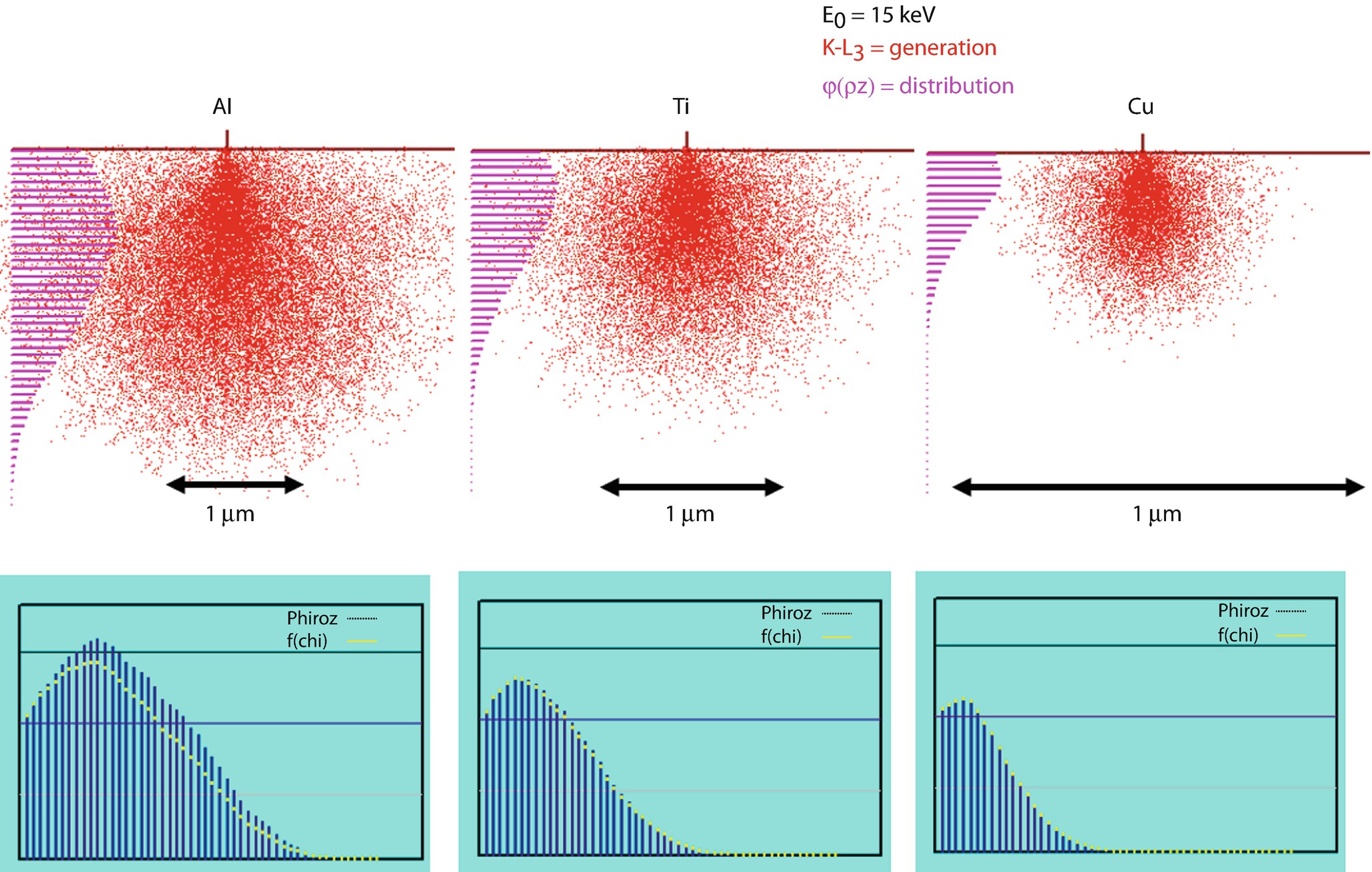
Monte Carlo simulations (Joy Monte Carlo) of X-ray generation at E ₀ = 15 keV for Al K-L₃, Ti K-L₃, and Cu K-L₃, showing (upper) the sites of X-ray generation (red dots) projected on the x-z plane, and the resulting φ(ρz) distribution. (lower) the φ(ρz) distribution is plotted with the associated f(χ) distribution showing the escape of X-rays following absorption

One can observe from ◘ Fig. 19.7 that there is a non-even distribution of X-ray generation with depth, z, for specimens with various atomic numbers and initial electron beam energies. This variation is illustrated by the histograms on the left side of the Monte Carlo simulations. These histograms plot the number of X-rays generated with depth into the specimen. In detail the X-ray generation for most specimens is somewhat higher just below the surface of the specimen and decreases to zero when the electron energy, E, falls below the critical excitation energy, E _c, of the characteristic X-ray of interest.

As illustrated from the Monte Carlo simulations, the atomic number of the specimen strongly affects the distribution of X-rays generated in specimens. These effects are even more complex when considering more interesting multi-element samples as well as the generation of L and M shell X-ray radiation.

◘ Figure 19.7 clearly shows that X-ray generation varies with depth as well as with specimen atomic number. In practice it is very difficult to measure or calculate an absolute value for the X-ray intensity generated with depth. Therefore, we follow the practice first suggested by Castaing (1951) of using a relative or a normalized generated intensity which varies with depth, called φ (ρz). The term ρz is called the mass depth and is the product of the density ρ of the sample (g/cm³) and the linear depth dimension, z (cm), so that the product ρz has units of g/cm². The mass depth, ρz, is more commonly used than the depth term, z. The use of the mass depth removes the strong variable of density when comparing specimens of different atomic number. Therefore it is important to recognize the difference between the two terms as the discussion of X-ray generation proceeds.

The general shape of the depth distribution of the generated X-rays, the φ (ρz) versus ρz curve, is shown in ◘ Fig. 19.8. The amount of X-ray production in any layer of the histogram is related to the amount of elastic scattering, the initial electron beam energy, and the energy of the characteristic X-ray of interest. The intensity in any layer of the φ (ρz) versus ρz curve is normalized to the intensity generated in an ideal thin layer, where “thin” is a thickness such that effectively no significant elastic scattering occurs and the incident electrons pass through perpendicular to the layer. As the incident beam penetrates the layers of material in depth, the length of the trajectory in each successive layer increases because (1) elastic scattering deviates the beam electrons out of the straight line path, which was initially parallel to the surface normal, thus requiring a longer path to cross the layer and (2) backscattering results in electrons, which were scattered deeper in the specimen, crossing the layer in the opposite direction following a continuous range of angles relative to the surface normal. Due to these factors, X-ray production increases with depth from the surface, ρz = 0, and goes through a peak, φ _m, at a certain depth ρR _m (see ◘ Fig. 19.8). Another consequence of backscattering is that surface layer production, φ ₀, is larger than 1.0 in solid samples because the backscattered electrons excite X-rays as they pass through the surface layer and leave the sample, adding to the intensity created by all of the incident beam electrons that passed through the surface layer. After the depth ρR _m, X-ray production begins to decrease with depth because the backscattering of the beam electrons reduces the number of electrons available at increasing depth ρz and the remaining electrons lose energy and therefore ionizing power as they scatter at increasing depths. Finally X-ray production goes to zero at ρz = ρR _x where the energy of the beam electrons no longer exceeds Ec.

../images/271173_4_En_19_Chapter/271173_4_En_19_Fig8_HTML.png — Fig. 19.8
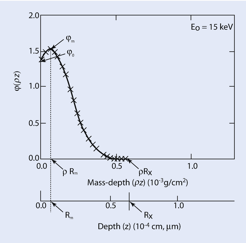
Schematic illustration of the φ(ρz) depth distribution of X-ray generation, with the definitions of specific terms: φ ₀, φ _m, ρR _m, R _m, ρR _X, and R _X

Now that we have discussed and described the depth distribution of the production of X-rays using the φ(ρz) versus ρz curves, it is important to understand how these curves differ with the type of specimen that is analyzed and the operating conditions of the instrument. The specimen and operating conditions that are most important in this regard are the average atomic number, Z, of the specimen and the initial electron beam energy, E ₀ chosen for the analysis. Calculations of φ(ρz) versus ρz curves have been made for this Appendix using the PROZA program (Bastin and Heijligers 1990). In ◘ Fig. 19.9, the φ(ρz) versus ρz curves for the K-L₃ X-rays of pure Al, Ti, and Cu specimens at 15 keV are displayed. The shapes of the φ(ρz) versus ρz curves are quite different. The φ₀ values, relative to the value of φ _m for each curve, increase from Al to Cu due to increased backscattering which produces additional X-ray radiation. On an absolute basis, the φ₀ value for Cu is smaller than the value for Ti because the overvoltage, U ₀, for the Cu K-L₃ X-ray at E ₀ = 15 keV is low (U ₀ = 1.67) and the energy of many of the backscattered electrons is not sufficient to excite Cu K-L₃ X-rays near the surface. The values of ρR _m and ρR _x decrease with increasing Z and a smaller X-ray excitation volume is produced. This decrease would be much more evident if we plotted φ(ρz) versus z, the linear depth of X-ray excitation, since the use of mass depth includes the density, which changes significantly from Al to Cu.

../images/271173_4_En_19_Chapter/271173_4_En_19_Fig9_HTML.png — Fig. 19.9
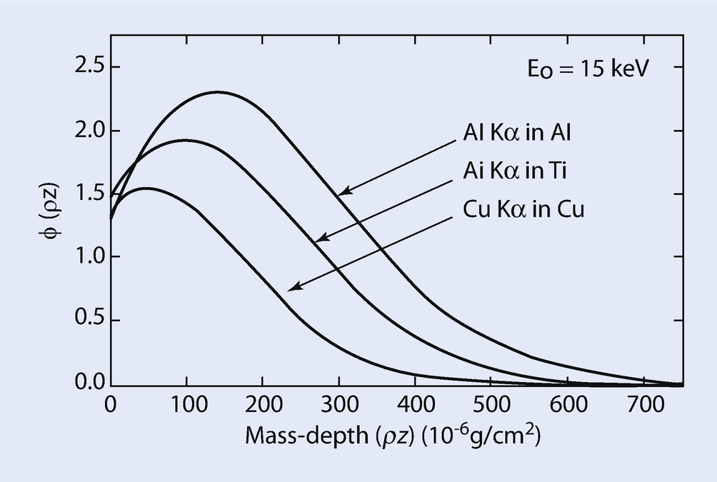
Calculated φ(ρz) curves for Al K-L₃ in Al; Ti K-L₃ in Ti; and Cu K-L₃ in Cu at E ₀ = 15 keV; calculated using PROZA

◘ Figure 19.10 shows calculated φ(ρz) versus ρz curves, using the PROZA program (Bastin and Heijligers 1990, 1991) at an initial beam energy of 15 keV for Al K-L₃ and Cu K-L₃ radiation for the pure elements Al and Cu. These curves are compared in ◘ Fig. 19.10 with calculated φ(ρz) versus ρz curves at 15 keV for Al K-L₃ and Cu K-L₃ in a binary sample containing Al with 3 wt % Cu. The φ ₀ value of the Cu K-L₃ curve in the alloy is smaller than that of pure Cu because the average atomic number of the Al – 3 wt % Cu sample is so much lower, almost the same as pure Al. In this case, less backscattering of the primary high energy electron beam occurs and fewer Cu K-L₃ X-rays are generated. On the other hand the Al K-L₃ φ(ρz) curves for the alloy and the pure element are essentially the same since the average atomic number of the specimen is so close to that of pure Al. Although the variation of φ(ρz) curves with atomic number and initial operating energy is complex, a knowledge of the pertinent X-ray generation curves is critical to understanding what is happening in the specimen and the standard for the element of interest.

../images/271173_4_En_19_Chapter/271173_4_En_19_Fig10_HTML.png — Fig. 19.10
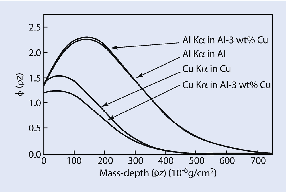
Calculated φ(ρz) curves for Al K-L₃ and Cu K-L₃ in Al, Cu, and Al-3wt%Cu at E ₀ = 15 keV; calculated using PROZA

The generated characteristic X-ray intensity, I_i gen, for each element, i, in the specimen can be obtained by taking the area under the φ(ρz) versus ρz curve, that is, by summing the values of φ(ρz) for all the layers Δ(ρz) in mass thickness within the specimen for the X-ray of interest. We will call this area “φ(ρz)_i,gen Area.” ◘ Table 19.3 lists the calculated values, using the PROZA program, of the φ(ρz)_i,gen Area for the 15 kev φ(ρz) curves shown in ◘ Fig. 19.10 (Cu K-L₃ and Al K-L₃ in the pure elements and Cu K-L₃ and Al K-L₃ in an alloy of Al – 3 wt % Cu and the corresponding values of φ ₀). A comparison of the φ(ρz)_i,gen Area values for Al K-L₃ in Al and in the Al – 3 wt % Cu alloy shows very similar values while a comparison of the φ(ρz)_i,gen Area values for Cu K-L₃ in pure Cu and in the Al – 3 wt % Cu alloy shows that about 17 % fewer Cu K-L₃ X-rays are generated in the alloy. The latter variation is due to the different atomic numbers of the pure Cu and the Al – 3 wt% Cu alloy specimen. The different atomic number matrices cause a change in φ ₀ (see ◘ Table 19.3) and the height of the φ(ρz) curves.

Table 19.3

Generated X-ray intensities in Al, Cu, and Al-3wt%Cu alloy, as calculated with PROZA (Bastin and Heijligers 1990, 1991)

Sample	X-ray	φ(ρz)_i,gen Area (cm²/g)	Atomic number factor, Z_i	φ ₀
Cu	Cu K-L₃	3.34 × 10⁻⁴	1.0	1.39
Al	Al K-L₃	7.85 × 10⁻⁴	1.0	1.33
Al-3wt%Cu	Cu K-L₃	2.76 × 10⁻⁴	0.826	1.20
Al-3wt%Cu	Al K-L₃	7.89 × 10⁻⁴	1.005	1.34

The atomic number correction, Z _i, can be calculated by taking the ratio of φ(ρz) _i,gen Area for the standard to φ(ρz) _i,gen Area for element i in the specimen. Pure Cu and pure Al are the standards for Cu K-L₃ and Al K-L₃ respectively. The values of the calculated ratios of generated X-ray intensities, pure element standard to specimen (Atomic number effect, Z _Al, Z _Cu) are also given in ◘ Table 19.3 As discussed above, it is expected that the atomic number correction for a heavy element (Cu) in a light element matrix (Al – 3 wt % Cu) is less than 1.0 and the atomic number correction for a light element (Al) in a heavy element matrix (Al – 3 wt % Cu) is greater than 1.0. The calculated data in ◘ Table 19.3 also show this relationship.

In summary, the atomic number matrix correction, Z _i, is equal to the ratio of Z _i,std in the standard to Z _i,unk in the unknown. Using appropriate φ(ρz) curves, correction Z _i can be calculated by taking the ratio of I _gen,std for the standard to I _gen,unk for the unknown for each element, i, in the sample. It is important to note that the φ(ρz) curves for multi-element samples and elemental standards which can be used for the calculation of the atomic number effect inherently contain the R and S factors discussed previously.

19.10.3.2 X-ray Absorption Effect, A

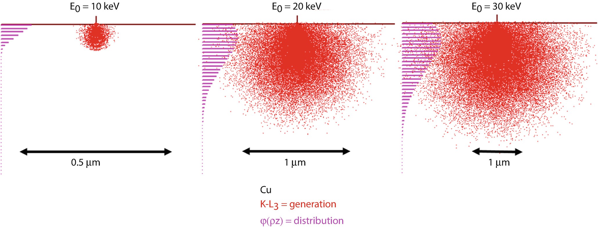
◘ Figure 19.11 illustrates the effect of varying the initial electron beam energy using Monte Carlo simulations on the positions where K-shell X-ray generation occurs for Cu at three initial electron energies, 10, 20, and 30 keV. This figure shows that the Cu characteristic X-rays are generated deeper in the specimen and the X-ray generation volume becomes larger as E ₀ increases. From these plots, we can see that the sites of inner shell ionizations which give rise to characteristic X-rays are created over a range of depth below the surface of the specimen.

../images/271173_4_En_19_Chapter/271173_4_En_19_Fig11_HTML.jpg — Fig. 19.11
Monte Carlo simulations (Joy Monte Carlo) of the X-ray generation volume for Cu K-L₃at E ₀ = 10 keV, 20 keV and 30 keV. The sites of X-ray generation (red dots) are projected on the x-z plane, and the resulting φ(ρz) distribution is shown

Created over a range of depth, the X-rays will have to pass through a certain amount of matter to reach the detector, and as explained in ► Chapter 4 (X-rays), the photoelectric absorption process will decrease the intensity. It is important to realize that the X-ray photons are either absorbed or else they pass through the specimen with their original energy unchanged, so that they are still characteristic of the atoms which emitted the X-rays. Absorption follows an exponential law, so as X-rays are generated deeper in the specimen, a progressively greater fraction is lost to absorption.

From the Monte Carlo plots of ◘ Fig. 19.11, one recognizes that the depth distribution of ionization is a complicated function. To quantitatively calculate the effect of X-ray absorption, an accurate description of the X-ray distribution in depth is needed. Fortunately, the complex three-dimensional distribution can be reduced to a one-dimensional problem for the calculation of absorption, since the path out of the specimen towards the X-ray detector only depends on depth. The φ(ρz) curves discussed previously give the generated X-ray distribution of X-rays in depth (See ◘ Figs. 19.8, 19.9, and 19.10). ◘ Figure 19.12 shows calculated φ(ρz) curves for Cu K-L₃ X-rays in pure Cu for initial beam energies of 10, 15, and 30 keV. The curves extend deeper (in mass depth or depth) in the sample with increasing E ₀. The φ ₀ values also increase with increasing initial electron beam energies since the energy of the backscattered electrons increases with higher values of E ₀.

../images/271173_4_En_19_Chapter/271173_4_En_19_Fig12_HTML.png — Fig. 19.12
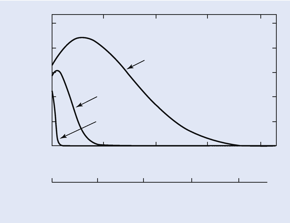
Calculated φ(ρz) curves for Cu K-L₃ in Cu at E ₀ = 10 keV, 20 keV, and 30 keV; calculated using PROZA

The X-rays which escape from any depth can be found by placing the appropriate path length in the X-ray absorption equation for the ratio of the measured X-ray intensity, I, to the generated X-ray intensity at some position in the sample, I ₀:

$I/{I}_0=\exp \left[-\left(\mu /\rho \right)\left(\rho t\right)\right]$

(19.18)

The terms in the absorption equation are (μ/ρ), the mass absorption coefficient; ρ, the specimen density; and t, the path length (PL) that the X-ray traverses within the specimen before it reaches the surface, z = ρz = 0. For the purpose of our interests, I represents the X-ray intensity which leaves the surface of the sample and I₀ represents the X-ray intensity generated at some position within the X-ray generation volume. Since the X-ray spectrometer is usually placed at an acute angle from the specimen surface, the so-called take-off angle, ψ, the path length from a given depth z is given by PL = z csc ψ, as shown in ◘ Fig. 19.13. When this correction for absorption is applied to each of the many layers Δ(ρz) in the φ(ρz) curve, a new curve results, which gives the depth distribution of emitted X-rays. An example of the generated and emitted depth distribution curves for Al K-L₃ at an initial electron beam energy of 15 keV (calculated using the PROZA program (Bastin and Heijligers 1990, 1991)) is shown in ◘ Fig. 19.14 for a trace amount (0.1 wt%) of Al in a pure copper matrix. The area under the φ(ρz) curve represents the X-ray intensity. The difference in the integrated area between the generated and emitted φ(ρz) curves represents the total X-ray loss due to absorption. The absorption correction factor in quantitative matrix corrections is calculated on the basis of the φ(ρz) distribution. ◘ Figure 19.5, for example, illustrates the large amount of Ni K-L₃ absorbed in the Fe-Ni alloy series as a function of composition.

../images/271173_4_En_19_Chapter/271173_4_En_19_Fig13_HTML.png — Fig. 19.13
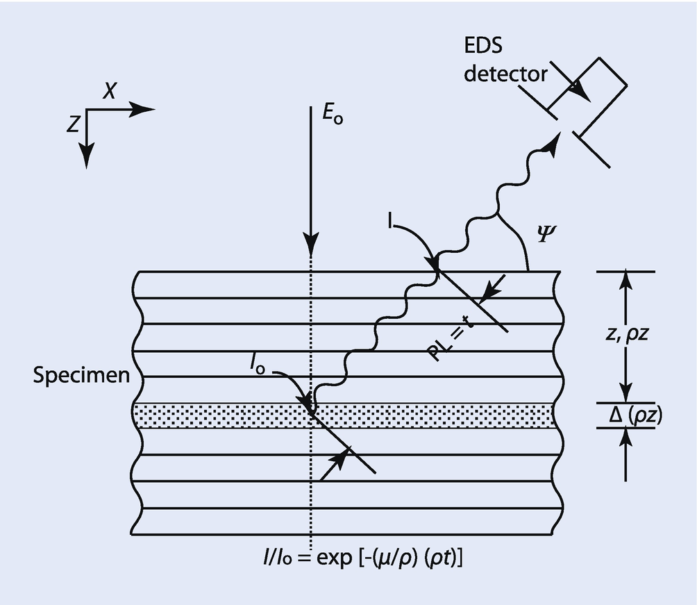
Schematic diagram of absorption in the measurement or calculation of the φ(ρz) curve for emitted X-rays. PL = path length, ψ = X-ray take-off angle (detector elevation angle above surface)

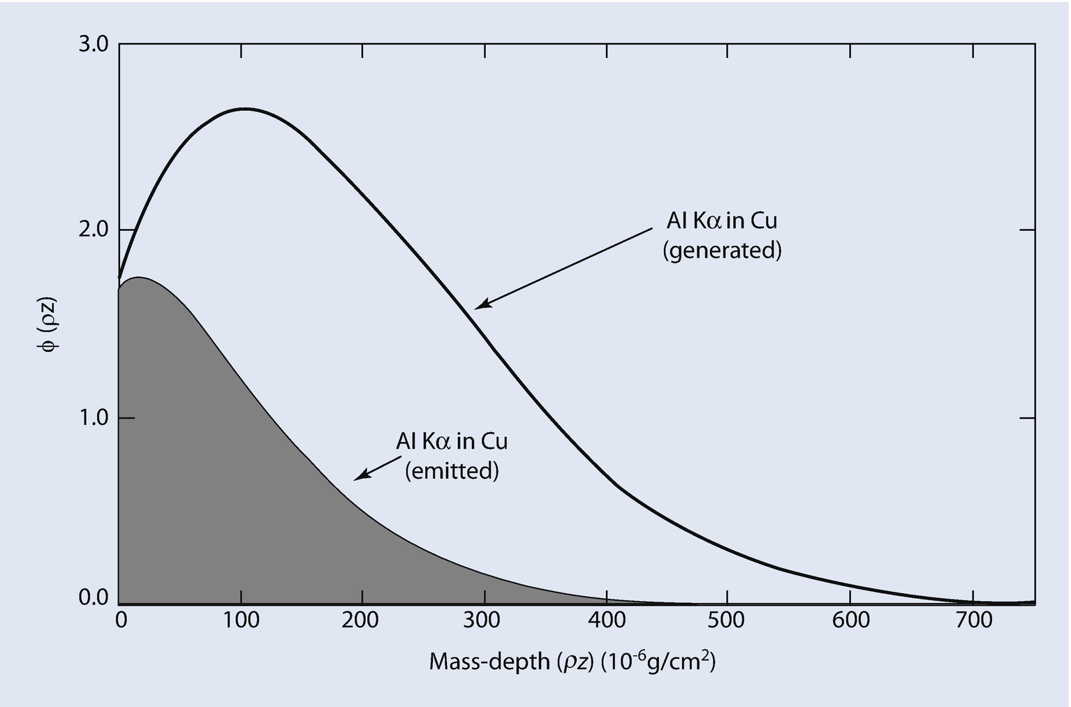
../images/271173_4_En_19_Chapter/271173_4_En_19_Fig14_HTML.png — Fig. 19.14
Calculated generated and emitted φ(ρz) curves for Al K-L₃ in a Cu matrix at E ₀ = 20 keV

X-ray absorption is usually the largest correction factor that must be considered in the measurement of elemental composition by electron-excited X-ray microanalysis. For a given X-ray path length, the mass absorption coefficient, (μ/ρ), for each measured characteristic X-ray peak controls the amount of absorption. The value of (μ/ρ) varies greatly from one X-ray to another and is dependent on the matrix elements of the specimen (see ► Chapter 4, “X-rays”). For example, the mass absorption coefficient for Fe K-L₃ radiation in Ni is 90.0 cm²/g, while the mass absorption coefficient for Al K-L₃ radiation in Ni is 4837 cm²/g. Using Eq. (19.18) and a nominal path length of 1 μm in a Ni sample containing small amounts of Fe and Al, the ratio of X-rays emitted at the sample surface to the X-rays generated in the sample, I/I₀, is 0.923 for Fe K-L₃ radiation but only 0.0135 for Al K-L₃ radiation. In this example, Al K-L₃ radiation is very heavily absorbed with respect to Fe K-L₃ radiation in the Ni sample. Such a large amount of absorption must be taken account of in any quantitative X-ray analysis scheme. Even more serious effects of absorption occur when considering the measurement of the light elements, for example, Be, B, C, N, O, and so on. For example, the mass absorption coefficient for C K-L radiation in Ni is 17,270 cm²/g, so large that in most practical analyses, no C K-L radiation can be measured if the absorption path length is 1 μm. Significant amounts of C K-L radiation can only be measured in a Ni sample within 0.1 μm of the surface. In such an analysis situation, the initial electron beam energy should be held below 10 keV so that the C K-L X-ray source is produced close to the sample surface.

As shown in ◘ Fig. 19.12, X-rays are generated up to several micrometers into the specimen. Therefore the X-ray path length (PL = t) and the relative amount of X-rays available to the X-ray detection system after absorption (I/I ₀) vary with the depth at which each X-ray is generated in the specimen. In addition to the position, ρz or z, at which a given X-ray is generated within the specimen, the relation of that depth to the X-ray detector is also important since a combination of both factors determine the X-ray path length for absorption. ◘ Figure 19.15 shows the geometrical relationship between the position at which an X-ray is generated and the position of the collimator which allows X-rays into the EDS detector. If the specimen is normal to the electron beam (◘ Fig. 19.15), the angle between the specimen surface and the direction of the X-rays into the detector is the take-off angle ψ. The path length, t = PL, over which X-rays can be absorbed in the sample is calculated by multiplying the depth in the specimen, z, where the X-ray is generated, by the cosecant (the reciprocal of the sine), of the take-off angle, ψ. A larger take-off angle will yield a shorter path length in the specimen and will minimize absorption. The path length can be further minimized by decreasing the depth of X-ray generation, R _x, that is by using the minimum electron beam energy, E ₀, consistent with the excitation of the X-ray lines used for analysis. ◘ Table 19.4 shows the variation of the path length that can occur if one varies the initial electron beam energy for Al K-L₃ X-rays in Al from 10 to 30 keV and the take-off angle, ψ = 15° and ψ = 60°.

../images/271173_4_En_19_Chapter/271173_4_En_19_Fig15_HTML.png — Fig. 19.15
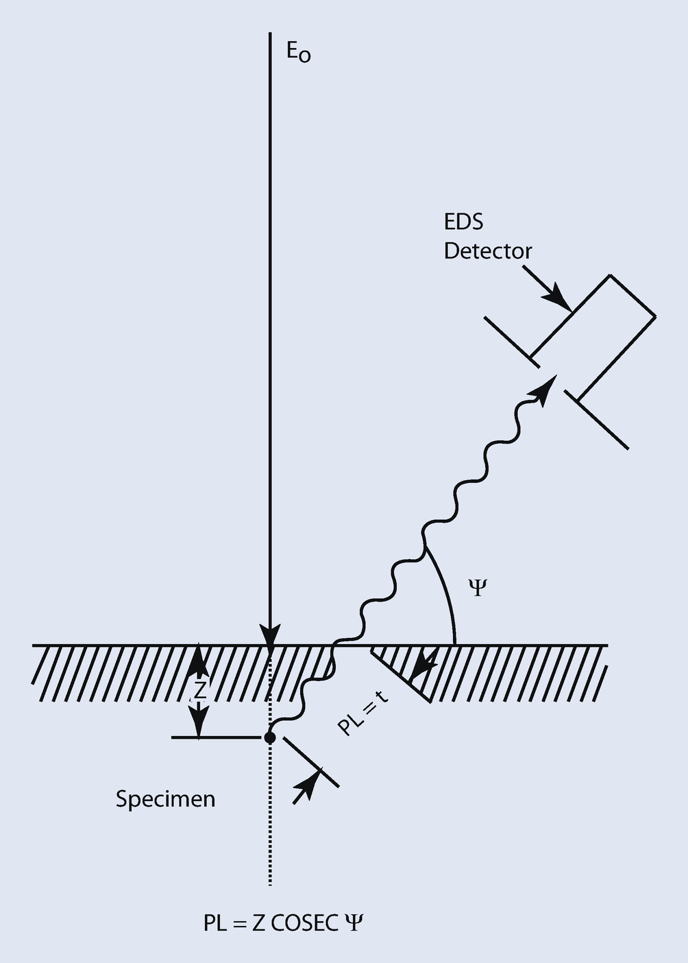
Schematic diagram showing the X-ray absorption path length in a thick, flat-polished sample: PL = absorption path length; ψ = X-ray take-off angle (detector elevation angle above surface)

Table 19.4

Path Length, PL, for Al K-L₃ X-rays in Al

E ₀	Take-Off Angle, ψ	R _x (μm)	Path Length, PL, (μm)
10	15	0.3	1.16
10	60	0.3	0.35
30	15	2.0	7.7
30	60	2.0	2.3

The variation in PL is larger than a factor of 20, from 0.35 μm at the lowest keV and highest take-off angle to 7.7 μm at the highest keV and lowest take-off angle. Clearly the analyst’s choices of the initial electron beam energy and the X-ray take-off angle have a major effect on the path length and therefore the amount of absorption that occurs.

In summary, using appropriate formulations for X-ray generation with depth or φ(ρz) curves, the effect of absorption can be obtained by considering absorption of X-rays from element i as they leave the sample. The absorption correction, Ai, can be calculated by taking the ratio of the effect of absorption for the standard, A _i,std, to X-ray absorption for the unknown, A _i,unk, for each element, i, in the sample. The effect of absorption can be minimized by decreasing the path length of the X-rays in the specimen through careful choice of the initial beam energy and by selecting, when possible, a high take-off angle.

19.10.3.3 X-ray Fluorescence, F

Photoelectric absorption results in the ionization of inner atomic shells, and those ionizations can also cause the emission of characteristic X-rays. For fluorescence to occur, an atom species must be present in the target which has a critical excitation energy less than the energy of the characteristic X-rays being absorbed. In such a case, the measured X-ray intensity from this second element will include both the direct electron-excited intensity as well as the additional intensity generated by the fluorescence effect. Generally, the fluorescence effect can be ignored unless the photon energy is less than 5 keV greater than the critical excitation energy, E _c.

The significance of the fluorescence correction, F _i, can be illustrated by considering the binary system Fe-Ni. In this system, the Ni K-L₃ characteristic energy at 7.478 keV is greater than the energy for excitation of Fe K radiation, E _c = 7.11 keV. Therefore, an additional amount of Fe K-L₃ radiation is produced beyond that due to the direct beam on Fe. ◘ Figure 19.5 shows the effect of fluorescence in the Fe-Ni system at an initial electron beam energy of 30 keV and a take-off angle, ψ, of 52.5°. Under these conditions, the atomic number effect, Z _Fe, and the absorption effect, A_Fe, for Fe K-L₃ are very close to 1.0. The measured k_Fe ratio lies well above the first approximation straight line relationship. The additional intensity is given by the effect of fluorescence. As an example, for a 10 wt% Fe – 90 wt% Ni alloy, the amount of iron fluorescence is about 25 %.

The quantitative calculation of the fluorescence effect requires a knowledge of the depth distribution over which the characteristic X-rays are absorbed. The φ(ρz) curve of electron-generated X-rays is the starting point for the fluorescence calculation, and a new φ(ρz) curve for X-ray-generated X-rays is determined. The electron-generated X-rays are emitted isotropically. From the X-ray intensity generated in each of the layers Δ(ρz) of the φ(ρz) distribution, the calculation next considers the propagation of that radiation over a spherical volume centered on the depth ρz of that layer, calculating the absorption based on the radial distance from the starting layer and determining the contributions of absorption to each layer (ρz) in the X-ray-induced φ(ρz) distribution. Because of the longer range of X-rays than electrons in materials, the X-ray-induced φ(ρz) distribution covers a much greater depth, generally an order of magnitude or more than the electron-induced φ(ρz) distribution. Once the X-ray-induced φ(ρz) generated distribution is determined, the absorption of the outgoing X-ray-induced fluorescence X-rays must be calculated with the absorption path length calculated as above.

The fluorescence factor, F _i, is usually the least important factor in the calculation of composition by evaluating the [ZAF] term in Eq. (19.17). In most analytical cases secondary fluorescence may not occur or the concentration of the element which causes fluorescence may be small. Of the three effects, Z, A, and F, which control X-ray microanalysis calculations, the fluorescence effect, F _i, can be calculated (Reed 1965), with sufficient accuracy so that it rarely limits the development of an accurate analysis.

Open Access This chapter is licensed under the terms of the Creative Commons Attribution-NonCommercial 2.5 International License (http://creativecommons.org/licenses/by-nc/2.5/), which permits any noncommercial use, sharing, adaptation, distribution and reproduction in any medium or format, as long as you give appropriate credit to the original author(s) and the source, provide a link to the Creative Commons license and indicate if changes were made.

The images or other third party material in this chapter are included in the chapter's Creative Commons license, unless indicated otherwise in a credit line to the material. If material is not included in the chapter's Creative Commons license and your intended use is not permitted by statutory regulation or exceeds the permitted use, you will need to obtain permission directly from the copyright holder.

References

Bastin GF, Heijligers HJM (1990) Quantitative electron probe microanalysis of ultralight elements (boron – oxygen). Scanning 12:225–236Crossref
Bastin GF, Heijligers HJM (1991) Quantitative analysis of homogeneous or stratified microvolumes applying the model “PAP”. In: Heinrich KFJ, Newbury DE (eds) Electron probe quantitation. Plenum Press, New York City, p 163
Castaing R (1951) “Application of electron probes to local chemical and crystallographic analysis” Ph.D. thesis, University of Paris. (English translation available from the Microanalysis Society at: ► http://www.microanalysissociety.org/
Heinrich KFJ, Myklebust RL, Rasberry SD, Michaelis RE (1971) Preparation and Evaluation of SRM’s 481 and 482 Gold-Silver and Gold-Copper Alloys for Microanalysis. U.S. Government Printing Office, Washington, DC. NBS Spec. Publ., pp 260–28
ISO GUM (2008). Guide to the Expression of Uncertainty in Measurement; Guide 98–3:2008: Geneva, Switzerland, Joint Group for Guides in Metrology, Working Group 1. ISO Central. Secretariat, Vernier, Geneva, Switzerland: International Organization for Standards
Marinenko R, Leigh S (2010) Uncertainties in electron probe microanalysis. Proc Eur Microbeam Anal Soc 7(1):012017
Marinenko R, Blackburn D, Bodkin J (1990) Glasses for Microanalysis: SRMs 1871-1875” National Institute of Standards and Technology (U.S.) Special Publication 260–112 (U.S. Gov. Printing Office, Washington) available at: ► http://www.nist.gov/srm/upload/SP260-112.PDF
Newbury DE, Swyt CR, Myklebust RL (1995) ‘Standardless’ quantitative electron probe microanalysis with energy-dispersive X-ray spectrometry: is it worth the risk? Anal Chem 67:1866Crossref
Pouchou J-L, Pichoir F (1991) Quantitative analysis of homogeneous or stratified microvolumes applying the model “PAP”. In: Heinrich KFJ, Newbury DE (eds) Electron probe quantitation. Plenum, New York, p 31Crossref
Reed SJB (1965) Characteristic fluorescence corrections in electron-probe microanalysis. Brit J Appl Phys 16:913Crossref
Saunders S, Karduck P, Sloof W (2004) Certified reference materials for micro-analysis of carbon and nitrogen. Microchim Acta 145:209Crossref
Yakowitz H (1975) Methods of quantitative analysis. In: Goldstein JI, Yakowitz H, Newbury DE, Lifshin E, Colby JW, Coleman JR (eds) Practical scanning electron microscopy. Plenum, New York, p 338

19. Quantitative Analysis: From k-ratio to Composition