Appendix A
A short course on path integrals
Path integrals are a powerful means of representing quantum theories, especially on surfaces of nontrivial topology. The introduction we present here is similar to that which the reader will find in any modern field theory text. We include it in order to emphasize certain ideas that we will need, such as the relation between the path integral and Hilbert space formalisms and the use of operator equations inside the path integral.
A.1 Bosonic fields
Consider first a quantum mechanics problem, one degree of freedom with Hamiltonian  , where

Throughout the appendix operators are indicated by hats. A basic quantity of interest is the amplitude to evolve from one q eigenstate to another in a time T,

In field theory it is generally convenient to use the Heisenberg representation, where operators have the time dependence

The state |q, t  is an eigenstate of
  (t),
(t),

In terms of the t = 0 Schrödinger eigenstates this is

In this notation the transition amplitude (A.1.2) is  qf, T \qi, 0.
By inserting a complete set of states, we can write the transition amplitude as a coherent sum over all states q through which the system might pass at some intermediate time t :

Divide the time interval further into N steps as in figure A.1,
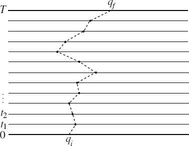
Fig. A.1. Transition amplitude broken down into time steps. The dashed line suggests a piecewise linear path, which is one of many ways to define path integration.

and corresponding to each intermediate time insert a complete set of states

Translate back to Schrödinger formalism and introduce an integral over intermediate momenta,
By commuting, we can always write  with all
  to the left and all to the right, so that

Use this to evaluate the matrix element in eq. (A.1.9). From expanding the exponential there will be terms of order  2 and higher that have to the left of ; drop these. Then to this order
  becomes

Thus

In the last line we have taken a formal → 0 limit, so the integral runs over all paths p(t), q(t) with given q(T) and q(0). This is the Hamiltonian path integral (or functional integral), the sum over phase space paths weighted by exp(iS/ ) with S the action in Hamiltonian form.
Let us integrate over p(t), making first the approximation that the integral is dominated by the point of stationary phase,

Solving for p in terms of q and  and recalling that L = p − H, the stationary phase approximation gives

Often the momentum integral is Gaussian,  , so that the stationary phase approximation is exact up to a normalization that can be absorbed in the measure [dq]. In fact, we can do this generally: because the relation (A.1.13) between p and is local, the corrections to the stationary phase approximation are local and so can be absorbed into the definition of [dq] without spoiling the essential property that [dq] is a product over independent integrals at each intermediate time. The result (A.1.14) is the Lagrangian path integral, the integral over all paths in configuration space weighted by exp(iS/), where now S is the Lagrangian action.
We have kept so as to discuss the classical limit. As → 0, the integral is dominated by the paths of stationary phase,  S/q(t) = 0, which is indeed the classical equation of motion. Henceforth, = 1.
The derivation above clearly generalizes to a multicomponent qi. One can always write a quantum field theory in terms of an infinite number of qs, either by making the spatial coordinate x discrete and taking a limit, or by expanding the x-dependence in terms of Fourier modes. Thus the above derivation of the path integral representation applies to bosonic field theory as well.
The derivation of the path integral formula treated the continuum limit → 0 rather heuristically. Renormalization theory is the study of this limiting process, and is rather well understood. The limit exists provided the Lagrangian satisfies certain conditions (renormalizability) and provided the coeffcients in the Lagrangian (bare couplings) are taken to vary appropriately as the limit is taken. The result is independent of various choices that must be made, including the operator ordering in the Hamiltonian, the precise definition of the measure, and the differences between regulators (the limit of piecewise linear paths suggested by the figure versus a frequency cutoff on the Fourier modes, for example).1 Being local effects these can all be absorbed into the bare couplings. Actually, we will evaluate explicitly only a few Gaussian path integrals. We use the path integral primarily to derive some general results, such as operator equations and sewing relations.
Relation to the Hilbert space formalism
Starting from the path integral one may cut it open to recover the Hilbert space of the theory. In equation (A.1.6), if one writes each of the amplitudes as a path integral one finds

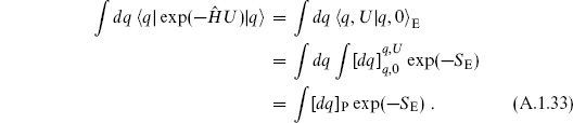
That is, the path integral on [0, T] breaks up into separate path integrals on [0,t] and [t, T], plus an ordinary integral over q(t). The boundary conditions on paths are denoted by super/subscripts. Note the restriction that T ≥ t ≥ 0. One can also replace the intermediate integral with a sum over any complete set of states. This cutting (or, inversely, sewing) principle is particularly useful on the surfaces of nontrivial topology that arise in string theory. There one may cut the surface open along many different closed curves; different choices give different Hilbert space representations of a given amplitude. This is known as world-sheet duality.
Consider now a path integral with the additional insertion of a factor of q(t), where 0 < t < T. Then, using the cutting relation (A.1.15),

Thus, q(t) in the functional integral translates into (t) in the matrix element. For a product of two insertions q(t)q(t′) (which is equal to q(t′)q(t), since these are simply variables of integration), where both t and t′ are in the range [0, T], one finds by the same method that

Here, T denotes the time-ordered product

Because of the way the path integral is built out of successive infinitesimal time slices, two or more insertions in the path integral will always correspond to the time-ordered product of operators in the matrix element.
The equation of motion is  Let us see how this works inside the path integral. Consider this equation in a path integral with other insertions
  ,
,

We have integrated by parts in the second line.2 If none of the fields in are at time t, the right-hand side vanishes and the equation of motion holds in the path integral. We therefore say that the equation of motion holds as an operator equation. This is a technique that we will use extensively: an operator equation is one which holds when inserted into any path integral that has no other fields coincident with those involved in the equation. Translating to Hilbert space language, we can use the other insertions to set up arbitrary initial and final states, so this corresponds to the ordinary notion that an operator equation is one that should hold for general matrix elements.
When additional insertions are present at t, operator equations inside the path integral hold only up to additional delta-function source terms. For example, let = q(t′)…, where t′ is near t and the other fields in ‘…’ are far away. Then eq. (A.1.19) becomes

This is an example of the Schwinger–Dyson equation, the equation of motion for the expectation value of a product of fields. The same result written as an operator equation is

As an explicit example, take the harmonic oscillator,

Then the operator equations we have derived are

and

In Hilbert space language these become

The first is the Heisenberg equation for the field operator, while the delta function in the second comes from the time derivative acting on the step functions in the time-ordered product,

Euclidean path integrals
In Schrödinger language, the time-ordered product (A.1.17) is

where t> is the greater of t and t′, and t< is the lesser. By the nature of the path integral, which builds amplitudes from successive time steps, the time differences multiplying H are always positive in amplitudes such as (A.1.27): one only encounters exp for positive Δt. Now continue analytically by uniformly rotating all times in the complex plane, t → e−i
 t for any phase 0 ≤
  ≤
≤  . The real part of the exponent is −E sinΔt, where E is the energy of the intermediate state. Because the Hamiltonian is bounded below for a stable system, the sum over intermediate states is safely convergent and no singularities are encountered — the continued amplitude is well defined.
Taking the times to be purely imaginary, t = −iu for real u, defines the Euclidean amplitudes, as opposed to the Minkowski amplitudes studied above:

is defined to be the continuation of

to t = −iu. One can repeat the derivation of the path integral representation for the Euclidean case, but the result is extremely simple: just replace t in the action with −iu,

The weight in the Euclidean path integral is conventionally defined to be exp(−SE), so the Euclidean action contains a minus sign,

Euclidean path integrals are usually the more well-defined, because the exponential of the action is damped rather than oscillatory. The Minkowski matrix elements can then be obtained by analytic continuation. In the text our main concern is the Euclidean path integral, which we use to represent the string S-matrix.
One is often interested in traces, such as

where the sum runs over all eigenvectors of and the Ei are the corresponding eigenvalues. In the q basis the trace becomes
In the last line, [dq]P denotes the integral over all periodic paths on [0, U]. An interesting variation on this is the integral over all antiperiodic paths:

Here  is the reflection operator, taking q to −q. We see that twisting the boundary conditions — for example, replacing periodic with antiperiodic — is equivalent to inserting an operator into the trace. Since 2 = 1, its eigenvalues are ±1. If we take the average of the periodic and antiperiodic path integrals, this inserts
  (1 + ), which projects onto the = +1 space:

In the same way, (periodic − antiperiodic) gives the trace on the = −1 space.
A minor but sometimes confusing point: if  is a Hermitean operator, the Euclidean Heisenberg operator (u) = exp
 exp(−u) satisfies

and so is not in general Hermitean. For this reason it is useful to define a Euclidean adjoint,

A Hermitean operator in the Schrödinger picture becomes Euclidean self-adjoint in the Euclidean Heisenberg picture.
Diagrams and determinants
The diagrammatic expansion is easily obtained from the path integral. This subject is well treated in modern field theory texts. We will only derive here a few results used in the text. For notational clarity we switch to field theory, replacing q(t) with a real scalar field  (t, x). Begin with the free action

where Δ is some differential operator. Consider the path integral with a source J( ), taking the Euclidean case to be specific,
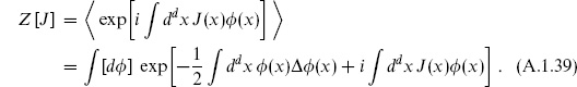
This is the generating functional for Euclidean Green’s functions. Taking functional derivatives with respect to J() pulls down factors of i() into the integral. Shifting to + iΔ−1J completes the square, leaving

In the second line, each derivative becomes iJ. Any functional of can be written

where  [J] is the (functional) Fourier transform of . By linearity one obtains

Expanding the exponential generates the diagrammatic expansion, all ways of contracting pairs of fields in . Also, when is a product of factors,  , we can separate

where /i acts only on i. The self-contractions are then the terms

Consider now the overall factor Z [0]. We assume that Δ is self-adjoint and so we expand () in a complete set of eigenfunctions  i():
i():

where

Define the path integral measure by

Then

The product of eigenvalues must be suitably regulated and renormalized. The value of 1 is usually given simply as (detΔ)−1/2, because a rescaling of Δ is equivalent to a rescaling of , the Jacobian for which can be absorbed into the bare couplings. (In free field theory, the only ‘coupling’ that would be renormalized would be a c-number constant in the Lagrangian density; we will see this appearing in the example.)
All of the above discussion extends readily to multicomponent qi or i. One case of interest is a complex scalar field. One can break this up into two real scalars, = 2−1/2(1 + i2), and the measure is [d d*] ≡ [d1 d2]. For complex fields, (A.1.48) becomes

One similarly finds for two real fields

This is a functional version of the delta-function integral

An example
As an example, we study the Euclidean transition amplitude for the harmonic oscillator,

where Sct is a cutoff-dependent piece to be determined later. To evaluate this, separate out the ‘classical’ part of q,

where

The boundary conditions on q′ are then

and the action separates

Here

The amplitude becomes

Expand in a complete set of eigenfunctions of  subject to the boundary condition (A.1.55),

The infinite product diverges. The Pauli–Villars regulator is a simple way to define it. Divide by the amplitude for a regulator oscillator of very high frequency Ω,

For j small, the terms in (A.1.60) are the same as those in (A.1.59b) up to a multiplicative constant, while for j large the product converges. The value of the product (A.1.60) is

This follows from a standard infinite product representation for the sinh. One can guess the result (A.1.61) by noting that it has the right poles and zeros in U, and the right value as U goes to zero.
Keeping only terms that are nonvanishing as Ω → ∞,

To get a finite answer as Ω → ∞, we need first to include a term Ω in the Lagrangian Lct, canceling the linear divergence in (A.1.62). That is, there is a linearly divergent bare coupling for the operator ‘1’. It may seem strange that we need to renormalize in a quantum mechanics problem, but the power counting is completely uniform with quantum field theory. The logarithmic divergence is a wavefunction renormalization. To determine the finite normalization, compare the path integral expression (A.1.62) to the canonical result as U → ∞. The U → ∞ amplitude is easily evaluated by inserting a complete set of states, since only the ground state |0 contributes in the limit:

On the other hand, the path integral expression (A.1.62) becomes


and

which is the correct result.
A.2 Fermionic fields
Consider the basic fermionic quantum system, two states |↑ and |↓ with raising operator  and lowering operator
  :
:

Amplitudes will be expressed as path integrals over the classical analogs of and . These are anticommuting c-numbers or Grassmann variables, elements  m and
m and  m of a Grassmann algebra

There is a natural notion of integration over Grassmann variables, the Berezin integral. Notice that if is a Grassmann variable then 2 = 0, and so the most general function of is of the form a + b. Define

Integrals of more general expressions are determined by requiring the integral to be linear and by defining d to anticommute with all Grassmann variables. The significance of the definition (A.2.3) is that the integral of a total derivative is zero:

For multiple Grassmann variables the integral is

where c is the coefficient of the highest term in the Taylor expansion of ,

Looking back on the discussion of the bosonic path integral, one sees that all of the properties of ordinary integrals that were used are also true for the Berezin integral: linearity, invariance (except for a sign) under change of order of integration, and integration by parts.3
In order to follow the bosonic discussion as closely as possible, it is useful to define states that are formally eigenstates of :

Define | to satisfy

The right-hand side is the Grassmann version of the Dirac delta function. It has the same properties as the ordinary delta function,

and

for arbitrary (). The state | is a left eigenstate with opposite sign,

as one verifies by taking the inner product of both sides with a general state |′. Note also that

One can verify this by taking the matrix element between arbitrary states ′| and |″ and evaluating the Grassmann integral.
The delta function has an integral representation

By expanding the inner product (A.2.8) in powers of ′ one obtains

and therefore

Using the further property that | is an eigenstate of , one obtains

This holds for any function with the prescription that it is written with the on the right.
We can now emulate the bosonic discussion, using the completeness relation (A.2.12) to join together successive time steps, with the result

The inconvenient sign in the integral representation has been offset by reversing the order of Grassmann integrations. A typical fermionic Hamiltonian is = m. The corresponding Lagrangian is L = i − H. For such first order Lagrangians the Hamiltonian and Lagrangian formulations coincide, and the result (A.2.17) is also the Lagrangian path integral.
There are two useful inner products for this system,

Inner product (A) is positive definite and gives  . It is the inner product for an ordinary physical oscillator. Inner product (B) is not positive, and it makes and Hermitean. It is the appropriate inner product for the Faddeev–Popov ghost system, as discussed in chapter 4. The derivation of the path integral was independent of the choice of inner product, but the relations (A.2.14) determine the expansion of | in basis states in terms of the inner product.
All of the discussion of the bosonic case applies to the fermionic path integral as well. The derivation is readily extended to multiple Fermi oscillators and to field theory. Renormalization theory works in the same way as for the bosonic path integral. Fermionic path integrals again satisfy cutting relations, which simply amount to taking one of the iterated integrals (A.2.17) and saving it for the end. Insertion of (t) and (t) in the path integral again gives the corresponding operator in the matrix element, and multiple insertions are again time-ordered. The path integral insertion


Note that a minus sign appears in the definition of time-ordering. The equations of motion and the Euclidean continuation work as in the bosonic case, but there is one important change. Consider a general operator ,

where i, j run over ↓ and ↑. Then by expanding | in terms of the basis states one finds

where the fermion number  has been defined to be even for |↓ and odd for |↑. In particular,

In contrast to the bosonic results (A.1.33) and (A.1.34), the periodic path integral gives the trace weighted by (–1) and the antiperiodic path integral gives the simple trace.
Feynman diagrams are as in the bosonic case, but the determinants work out differently. Consider

where we have again switched to the notation of field theory. Expand in eigenfunctions of Δ, and in eigenfunctions of ΔT,

Define [dd] = Πi didi. Then

Similarly, one finds for a single field that

where Δ must be antisymmetric. These fermionic path integrals are just the inverse of the corresponding bosonic integrals.
For finite-dimensional integrals we have to be careful about 2s,

Curiously, we can be more cavalier for functional determinants, where these can be eliminated by rescaling the fields. Bosonic path integrals actually give the absolute values of determinants, while fermionic path integrals give the determinant with a sign that depends on the precise order of Grassmann factors in the measure. We will fix the sign by hand.4
If Δ has zero eigenvalues, the path integral vanishes in the fermionic case and diverges in the bosonic case. When this occurs there is always a good reason, as we will see in practice, and the integrals of interest will have appropriate insertions to give a finite result.
A useful result about Berezin integrals: from the definition it follows that if ′ = a then d′ = a−1d. That is, the Jacobian is the inverse of the bosonic case. More generally, with bosonic variables i and Grassmann variables j, under a general change of variables to  the infinitesimal transformation of the measure has an extra minus sign,

Exercises
A.1 (a) Evaluate the path integral (A.1.33) for the harmonic oscillator by expanding [dq]P in a set of periodic eigenfunctions (not by inserting the result already obtained for the transition function into the left-hand side). Compare with an explicit evaluation of the sum over states (A.1.32).
(b) Do the same for the antiperiodic path integral (A.1.34).
A.2 Consider two harmonic oscillators of the same frequency, and form the complex coordinate q = 2−1/2(q1 + iq2). Evaluate the following path integral on [0, U] by using a suitable mode expansion:

where the integral is to run over all paths such that q(U) = q(0)ei. Again compare with the answer obtained by summing over states: it is useful here to form complex combinations of oscillators, a1 ± ia2. This is a more exotic version of exercise A.1, and arises in various string theories such as orbifolds.
A.3 Consider a free scalar field X in two dimensions, with action

Evaluate the path integral with both coordinates periodic,

[Expanding the spatial dependence in Fourier modes, the answer takes the form of an infinite product of harmonic oscillator traces.]
A.4 Consider a free particle on a circle,
By means of path integrals, evaluate  . Be careful: there are topologically inequivalent paths, distinguished by the number of times they wind around the circle.
A.5 The fermionic version of exercise A.1: evaluate the fermionic path integral (A.2.23) and the corresponding antiperiodic path integral by using a complete set of periodic or antiperiodic functions, and compare with the sum over states.
__________
1 As another example, one can freely rescale fields. The Jacobian is formally a product of separate Jacobians at each point; its logarithm is therefore a sum of a local expression at each point. Regulated, this is just a shift of the bare couplings.
2 The functional derivative is defined as
It can be regarded as the limit of the ordinary derivative
In particular, one can integrate a functional derivative by parts, as for an ordinary derivative.
3 It is not useful to think of  d as an integral in any ordinary sense: it is simply a linear mapping from functions of to the complex numbers. Since it shares so many of the properties of ordinary integrals, the integral notation is a useful mnemonic.
4 A fine point: when the world-sheet theory is parity-asymmetric, even the phase of the path integral is ambiguous. The point is that Δ is not Hermitian in this case, because the Euclidean adjoint includes a time-reversal (which is the same as a parity flip plus Euclidean rotation). One must instead take the determinant of the Hermitian operator Δ Δ, which determines that of Δ only up to a phase. We will encounter this in section 10.7, for example, where we will have to check that there is a consistent definition of the phase.