The Princeton Guide to Evolution

IV.1

Genetic Drift

Philip Hedrick

OUTLINE

1. Genetic drift

2. Effective population size

3. Neutral theory

4. Coalescence

5. Future directions

Genetic drift is the chance change in genetic variation resulting from small population size. The effective population size, which can incorporate unequal numbers of male and female parents, variation in progeny number, or variation in numbers over different generations, is a useful concept for understanding genetic drift. The neutral theory incorporates the effects of genetic drift and mutation to understand the amount and pattern of molecular genetic variation. Coalescent approaches provide a way to estimate the past population size and other evolutionary factors.

GLOSSARY

Coalescence. The point or event in the past at which common ancestry occurs for two alleles at a gene because of genetic drift.

Effective Population Size (N_e). An ideal population that incorporates such factors as variation in the sex ratio of breeding individuals, the offspring number per individual, and numbers of breeding individuals in different generations.

Founder Effect. Impact on genetic variation in a population when it grows from a few founder individuals.

Genetic Bottleneck. A period during which only a few individuals survive and become the only ancestors of the future generations of the population.

Genetic Drift. Chance changes in allele frequencies that result from small population size.

Linkage Disequilibrium. Statistical association of alleles at different loci.

Molecular Clock. A constant rate of genetic substitution over time for molecular variants.

Neutral Theory. The theory that states that genetic change is primarily the result of mutation and genetic drift, and that different molecular genotypes are neutral with respect to each other.

Population. A group of interbreeding individuals existing together in time and space.

The primary goals of population genetics are to understand the genetic factors determining evolutionary change and stasis and the amount and pattern of genetic variation within and between populations (Hartl and Clark 2007; Hedrick 2011). In the 1920s and 1930s, shortly after widespread acceptance of Mendelian genetics, the theoretical basis of population genetics was developed by Ronald A. Fisher, J.B.S. Haldane, and Sewall Wright. As they showed, the amount and kind of genetic variation within and between populations are potentially affected by selection, inbreeding, genetic drift, gene flow, mutation, and recombination. Fisher thought that selection was most important and that genetic drift played only a minor role in evolutionary genetics, whereas Wright advocated a central role for genetic drift as well as selection, and in fact, genetic drift was sometimes called the “Sewall Wright effect.”

Generally, these evolutionary factors can have particular effects; for example, genetic drift and inbreeding can be considered to always reduce the amount of variation, and mutation to always increase it. Other factors, such as selection and gene flow, can either increase or reduce genetic variation, depending on the particular situation. In addition, the factors other than genetic drift generally have deterministic effects; for example, given certain relative fitness values for genotypes, selection results in a predictable genetic change. Genetic drift is different from these other factors in that it has a nondeterministic or stochastic effect; that is, genetic changes resulting from genetic drift are random in direction.

The development of population molecular data in the late 1960s, DNA sequence data in the 1980s, and genomic data in recent years have revolutionized population genetics and produced many new questions and some answers. Population genetics and its evolutionary interpretations provided a fundamental context in which to interpret this new molecular genetic information. For example, Motoo Kimura in 1968 introduced the neutral theory of molecular evolution that assumes that genetic variation results primarily from a combination of mutation-generating variation and its elimination by genetic drift (Kimura 1983). This theory is called neutral because allele and genotype differences at a gene are selectively neutral with respect to each other. This theory is consistent with many observations of molecular genetic variation.

1. GENETIC DRIFT

Before we discuss genetic drift, let us first define the evolutionary or genetic connotation of the term population. As a simple ideal, a population is group of interbreeding individuals that exists together in time and space. Genetic drift refers to chance changes in allele frequency that result from the sampling of gametes from generation to generation in a population. Since the beginning of population genetics, there has been controversy concerning the importance of genetic drift. Part of this controversy has resulted from the large numbers of individuals observed in many natural populations, large enough to think that chance effects would be small in comparison to the effects of other factors, such as selection and gene flow.

Under certain conditions, a population may be so small that genetic drift is significant even for loci with sizable selective effects, or when there is significant gene flow. For example, some populations may be continuously small for relatively long periods of time because of limited resources in the populated area. In addition, some populations may have intermittent small population sizes. Examples of such episodes are the overwintering loss of population numbers in many invertebrates, and epidemics that periodically decimate populations of both plants and animals. Such population fluctuations generate genetic bottlenecks, or periods during which only a few individuals survive and become the only ancestors of the future generations of the population.

Small population size is also important when a population grows from a few founder individuals, a phenomenon termed founder effect. For example, many island populations appear to have started from a very small number of individuals. If a single female who was fertilized by a single male founds a population, then only four genomes (assuming a diploid organism), two from the female and two from the male, can start a new population. In plants, a whole population can be initiated from a single seed—only two genomes, if self-fertilization occurs. As a result, populations descended from a small founder group may have low genetic variation, or by chance have a high or low frequency of particular alleles.

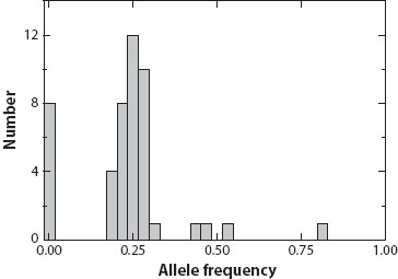
Kalinowski et al. (2010) provided an excellent example of a founder effect in lake trout that invaded Swan Lake in Montana in the late 1990s. The number of founders was not observed, but samples taken less than a decade after they invaded provided a genetic signal. First, a limited number of alleles at 11 microsatellite loci, only four or fewer alleles with a frequency greater than 2 percent, were observed in the founders, while samples from the putative source, Flathead Lake, averaged more than 12 alleles per locus. Second, the allele frequencies in Swan Lake sample, clustered around 0.25, 0.5, and 0.75 (one, two, or three out of four copies) (figure 1), whereas many other alleles observed in Flathead Lake were not found. This suggests that the population was founded primarily by only two individuals, only four genomes, and that the chance effects of this founding event are reflected in the allele frequencies.

Figure 1. Histogram of the number of the alleles with different frequencies for the 11 microsatellite loci in lake trout from Swan Lake. (After Kalinowski et al. 2010.)

Another situation in which small population size is of great significance is one in which the population (or species) in question is one of the many threatened or endangered species (Allendorf et al. 2013). For example, all approximately 500 whooping cranes alive today descend from only 20 whooping cranes that were alive in 1920 because only a few had survived hunting and habitat destruction. All 200,000 northern elephant seals alive today descend from as few as 20 that survived nineteenth-century hunting on Isla Guadalupe, Mexico. Further, all the living individuals of some species are descended from a few founders that were brought into captivity to establish a protected population, such as Przewalski’s horses (13 founders), California condors (13 founders), black-footed ferrets (6 founders), Galápagos tortoises from Española Island (15 founders), and Mexican wolves (7 founders).

All these examples of restricted population size can have the same general genetic consequence: a small population size causes chance alterations in allele frequencies. Genetic drift has the same expected effect on all loci in the genome. In a large population, on average, only a small chance change in the allele frequency will occur as the result of genetic drift. On the other hand, if the population size is small, then the allele frequency can undergo large fluctuations in different generations in a seemingly unpredictable pattern and can result in chance fixation or loss of an allele. These effects describe both the impact of genetic drift over all the different loci (the total genome) in a given population and the impact of genetic drift at a single locus over replicate populations, as discussed below.

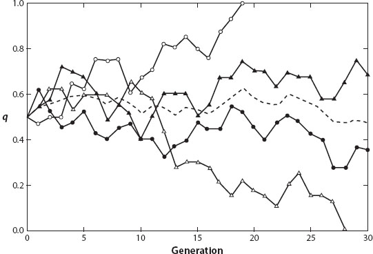
Figure 2 illustrates the type of allele frequency change expected in a small diploid population with two alleles, A₁ and A₂ (Hedrick 2011). This example uses Monte Carlo simulation with uniform random numbers to imitate the change in frequency of allele A₂ (q) in four replicate populations. Here the solid lines are the four replicates of a diploid population of size N = 20 (2N = 40), and the broken line is the mean frequency of A₂ over the four replicates. All the replicates were initiated with the frequency of A₂ equal to 0.5. One of these simulated replicates went to fixation for A₂ in generation 19, and another lost A₂ in generation 28. The other two replicates were still segregating for both alleles at the end of 30 generations. As shown here, genetic drift may cause large and erratic changes in allele frequency in a rather short time.

Figure 2. Frequency of allele A₂ over 30 generations for four replicates (solid lines) of a population of size 20. The mean frequency of allele A₂ is indicated by the broken line. (After Hedrick 2011.)

On the other hand, the mean frequency of A₂ for the four replicates varied much less: it ranged from 0.625 in generation 19 to 0.475 in generation 30 but was generally near the initial frequency of 0.5. If there are enough replicate populations, then there is no expected change in the mean allele frequency from genetic drift, so that

where ¯q_t is the mean frequency of A₂ in generation t over all replicates (0.5 in this example). The constancy of the mean frequency occurs because the increases in allele frequency in some replicates are cancelled by reductions in allele frequency in other replicates.

Individual replicates eventually either go to fixation for A₂ (q = 1) or to loss of A₂ (q = 0). The proportion of populations expected to go to fixation for a given allele is equal to the initial frequency of that allele (see chapter V.1). In other words, if the initial frequency of A₂ is q₀, and assuming that genetic drift is the only evolutionary factor influencing it, then the probability of fixation of that allele, u(q) (proportion of replicate populations eventually fixed for it), is

For example, if the initial frequency of A₂ is 0.1, only 10 percent of the time will a population become fixed for that allele. On the other hand, if the initial frequency of A₂ is 0.9, 90 percent of the time it will become fixed. This can be understood intuitively because the amount of change necessary to go from a frequency of 0.1 to 1.0 is much greater than from 0.9 to 1.0. This finding is a fundamental aspect of the neutrality theory used in molecular evolution; that is, without differential selection, the probability of fixation of a given allele is equal to its initial frequency.

Because the mean allele frequency does not change but the distribution of the allele frequencies over replicate populations does, the overall effect of genetic drift is best understood by examining the heterozygosity (or the variance) of the allele frequency over replicate populations (or multiple, independent loci). This is because the heterozygosity decreases as allele frequencies get closer to 0 or 1, a general consequence of genetic drift as shown in figure 2. The simplest approach to understanding the general effect of genetic drift is to examine the relationship between the heterozygosity over time in a small diploid population of size N. The expression giving this relationship is

where t is the number of generations and N is the effective population size (see below). For example, we can predict how much the level of heterozygosity is reduced after 30 generations from genetic drift with an effective population size of 20. In this case, H_t/H₀ = e^-30/40 = 0.472, or the level of heterozygosity is predicted to be reduced by 52.8 percent. Although we had only four replicate populations in the example in figure 2, by generation 30, two replicates had become fixed, reflecting this expectation.

If we go back to the lake trout example of Kalinowski et al. (2010), the average heterozygosities in the source Flathead Lake and in Swan Lake are 0.88 and 0.68, respectively. Let us assume only one generation of genetic drift (t = 1), because around 7000 lake trout were already present in Swan Lake only 10 years (two generations) after their discovery there. Therefore, H₀ = 0.88 and H₁ = 0.68 (assuming t = 1), and solving for the equation above for N, then

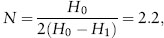
again suggesting that there were primarily two founders that established this population.

2. EFFECTIVE POPULATION SIZE

The number of breeding individuals in a population may be much less than the total number of individuals in an area, the census population size, but even the breeding population number might not be indicative of the population size appropriate for evolutionary considerations. For example, other factors, such as variation in the sex ratio of breeding individuals, the offspring number per individual, and numbers of breeding individuals in different generations, may be evolutionarily important. As a result, the effective population size (N_e), a theoretical concept that incorporates variation in these factors and others, is quite useful (Charlesworth 2009).

The concept of the effective population size makes it possible to consider an ideal population of size N in which all parents have an equal expectation of being the parents of any progeny individual. In general, the effect of genetic drift in a diploid population is a function of the reciprocal of twice the effective population size, 1/(2N_e). If N_e is large, then this value is small and there is little genetic drift influence. Or, if N_e is small, then this value is larger and genetic drift may be important.

A straightforward approach often used to tell the impact of various factors on the effective population size is the ratio of the effective population size to breeding (or sometimes census) population size N, that is, N_e/N. Sometimes, this ratio is only around 0.1 to 0.25, indicating that the effective population size may be much less than the number of breeding individuals (Palstra and Ruzzante 2008).

Assuming there are N individuals in the population, N_f is the number of females, and N_m is the number of males (N = N_f + N_m), then the effective population size becomes

If there are equal numbers of females and males, N_f = N_m = ½N, then N_e = N; however, in some species, the numbers of females and males are often unequal. Frequently, the number of breeding males is smaller than the number of breeding females (N_m < N_f), because some males mate more than once.

Let us assume the most extreme situation possible, one male mates with all the females in a colony or harem, as is thought to occur in some vertebrate populations where males control female harems, such as elephant seals. In this case, the expression above becomes

Note that the maximum value of this expression, when N_f becomes large, is 4.0. In other words, because each sex must contribute half the genes to the progeny, restricting the number of breeding individuals of one sex can greatly reduce the effective population size.

There may be a nonrandom distribution of progeny (gametes) per parent because of genetic, environmental, or accidental factors. For example, some birds have strongly determined numbers of eggs in a clutch, so the variance of egg number in a clutch may be near zero. Or, in some human populations, a relatively uniform number of offspring per parent may lower variation because of efforts to control population growth. On the other hand, if whole clutches or broods survive or perish as a group, then the variance of progeny number may be larger. Even more extreme, in some organisms with very high reproductive potential, a substantial proportion of the progeny may come from only a few highly successful parents.

To examine the impact of variance in the number of offspring, let us assume that the population is not changing in size (the number of progeny per individual is two), then the effective population size is

where V is the variance in the number of progeny. If V = 2 (the variance equals the mean number of progeny of two), then N_e≈N. If V = 0, where there are exactly two progeny from each individual, then N_e≈2N or N_e/N≈2. Therefore, if V is kept low, the effects of small population size can be avoided to some extent, and the effective population size may actually be larger than the breeding or census number; often, however, the variance in progeny number is larger than the mean, and as a result, N_e /N is lower than unity. In some organisms, such as many shellfish or fish, there may be very high variance in reproduction, where, in a given year, most of the recruited young may be from a few parents. For example, if V = 40, then N_e/N ≈ 0.1.

When the effective population size varies greatly in size in different generations, it can have a large impact on the overall effective population size. The variation in population size can result from regular cyclic variation in population numbers, periodic decimation of the population because of disease or other factors, or seasonal variation in population numbers. When this occurs, the lowest population numbers determine, to a large extent, the overall effective population size, because after these bottlenecks, all remaining individuals are descendants of the bottleneck survivors.

The effective population size over t generations becomes approximately

where N_e.i is the effective population size in generation i. For example, assume that the population in three subsequent generations has effective population sizes of 10, 100, and 1,000. Applying the expression above gives the effective population size of 27.0, closest to the lowest of the three populations sizes in different generations, and much smaller than the mean census number of 370 and N_e/N = 0.073, a quite low proportion.

The effective population size can be estimated using demographic information such as sex ratios, variance in progeny production, and variance in N_e over time. In addition, N_e can be estimated from observations of the effect of genetic drift on genetic variation over time in a population. For example, in a small population, both the change in allele frequency between generations and loss of heterozygosity are expected to be much higher than in a large population. Another approach is to measure the linkage disequilibrium, or the statistical association of alleles at different loci, as an indicator of the effective population size. For large populations, very little association of alleles at different loci is expected (unless they are tightly linked), whereas for small populations, large associations can be generated by chance.

The most comprehensive estimate of N_e using linkage disequilibrium is by Tenesa et al. (2007) who used data from about 1 million SNPs (single nucleotide polymorphisms) in four human samples from Nigeria, Europe, China, and Japan that provided about 20 million closely linked SNP pairs. Figure 3 gives the estimates of N_e from these data for each of the 22 autosomes and the X chromosome. The average N_e estimates over all chromosomes for the Nigerian, European, Chinese, and Japanese samples are 6286, 2772, 2620, and 2517, respectively. The European, Chinese, and Japanese populations have very similar N_e estimates for nearly all the chromosomes, and the overall N_e estimate for the African sample is about 2.4 times as large. This pattern is consistent with the hypothesis that the non-African populations descended from a migrant African population that represented a subset of the variation present in Africa at that time.

Figure 3. The effective population size for each chromosome estimated from linkage disequilibrium between about 20 million closely linked SNPs in four human populations. (After Tenesa et al. 2007.)

3. NEUTRAL THEORY

Neutral theory generally assumes that selection plays a minor role in determining the maintenance of molecular variants and proposes that different molecular genotypes have almost identical relative fitnesses; that is, they are neutral with respect to each other. The actual definition of selective neutrality depends on whether changes in allele frequency are determined primarily by genetic drift. In a simple example, if s is the selective difference between two alleles at a locus, and if s < 1/(2N_e), the alleles are said to be neutral with respect to each other because the impact of genetic drift is larger than selection.

The neutral theory is also consistent with a molecular clock; that is, there is a constant rate of substitution over time for molecular variants (see chapter II.3). To illustrate the mathematical basis of the molecular clock, let us assume that mutation and genetic drift are the determinants of changes in frequencies of molecular variants. Let the mutation rate to a new allele be u so that in an effective population of size 2N (we will drop the subscript e in this discussion and just assume N_e = N), there are 2Nu new mutants per generation. The probability of chance fixation of a new neutral mutant is 1/(2N) (the initial frequency of the new mutant). Therefore, the rate of allele substitution k is the product of the number of new mutants per generation and their probability of fixation, or

In other words, this elegant prediction from the neutral theory is that the rate of substitution is equal to the mutation rate at the locus and constant over time. Note that substitution rate is independent of the effective population size, a fact that may initially be counterintuitive. This independence occurs because in a smaller population there are fewer mutants; that is, 2Nu is smaller, but the initial frequency of these mutants is higher, increasing the probability of fixation, 1/(2N), by the same magnitude by which the number of mutants is reduced. This simple, mathematical prediction and others from the neutral theory provide the basis for the most important developments in evolutionary genetics in recent decades.

One of the appealing aspects of the neutral theory is that if it is used as a null hypothesis, predictions about the magnitude and pattern of genetic variation are possible. Initially, molecular genetic variation was found consistent with that predicted from neutrality theory. In recent years, examination of neutral theory predictions in DNA sequences has allowed tests of the cumulative effect of many generations of selection and a number of examples of selection on molecular variants have been documented.

If it is assumed that an equilibrium exists between mutation producing new alleles and genetic drift eliminating them, then

the equilibrium heterozygosity for the neutral model. Note that for this equilibrium, the allele frequencies, and even the identity of the alleles, are constantly changing as new mutants are generated and old mutants impacted by genetic drift, and it is only the distribution of alleles that remains more or less constant. This equation predicts that as 4N_eu increases, the amount of heterozygosity will also increase; therefore, neutrality predicts that an increase in either effective population size or mutation rate will result in an increase in heterozygosity. Surveys of microsatellite loci, which have a high mutation rate, generally have a high heterozygosity, consistent with predictions from the neutral theory; for example, some microsatellite loci have mutation rates of u = 10^-4, and if N_e = 10,000, then H_e = 0.8, as often found for microsatellite loci.

4. COALESCENCE

Traditionally, population genetics examines the impact of various evolutionary factors on the amount and pattern of genetic variation in a population and how these factors influence the future potential for evolutionary change. Generally, evolution is conceived of as a forward process, examining and predicting the future characteristics of a population; however, rapid accumulation of DNA sequence data over the past two decades has changed the orientation of much of population genetics from a prospective one, investigating the factors involved in observed evolutionary change, to a retrospective one, inferring evolutionary events that have occurred in the past. That is, understanding the evolutionary causes that have influenced the DNA sequence variation in a current sample of individuals, such as the demographic and mutational history of the ancestors of the sample, has become the focus of much population genetics research.

When DNA variation is being determined in a population at a given locus, a sample of alleles is examined. Each one of these alleles can have a different history, ranging from descending from the same ancestral allele, that is, identical by descent, in the previous generation to descending from the same ancestral allele many generations before. The point at which this common ancestry for two alleles occurs is called coalescence. If one goes back far enough in time in the population, all alleles in the sample will coalesce into a single common ancestral allele. Research using the coalescent approach is the most dynamic area of theoretical population genetics because it is widely used to analyze DNA sequence data in populations and species.

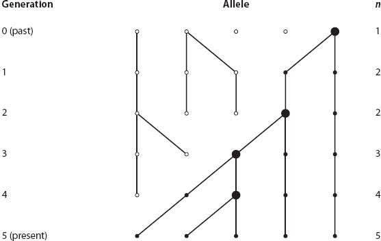
To illustrate the coalescent process, figure 4 gives a hypothetical example of the ancestry of five alleles sampled in the present generation, generation 5. If we go down in figure 4, forward in time, we can see the effect of genetic drift in a very small population: some alleles are lost (such as the middle allele in the first generation because it has no descendants), and some alleles increase in frequency, such as the right-hand allele (it has two descendants in the second generation). After five generations, only the right-hand allele remains, the other four original alleles have been lost. Of course, if the population size were larger, coalescent events from genetic drift would be less frequent and spaced out over many generations.

Figure 4. The ancestry of five alleles sampled in the present generation. If we go backward in time, bottom to top, we see the effects of genetic drift in a very small population resulting in coalescence in a single allele in generation 0 (n is the number of ancestral alleles in a given generation). (After Hedrick 2011.)

The theory of coalescence allows us to examine only the alleles ancestral to those sampled in the present generation. If we go up in figure 4, back in time, we see that the five alleles sampled in the present generation 5 are descended from four alleles in generation 4. In other words, there is a coalescent event because two alleles in generation 5 are descended from the same ancestral allele in generation 4, indicated by a larger circle. If we continue up the figure, the number of ancestral alleles declines because of three additional coalescent events, until only one ancestral allele remains in generation 0. Notice that other alleles were present in the past, but they have left no descendants in the present-day sample.

In this example, only genetic drift is assumed to influence the alleles, and mutation is not included. If mutation is included, observed alleles that have a common ancestor may actually have somewhat different DNA sequences. Coalescent theory and molecular data allow estimation of past events; for example, the past effective population size thousands of generations ago can be estimated using contemporary molecular data.

5. FUTURE DIRECTIONS

Genomic data from many individuals in a population or species and theoretical coalescent approaches will provide new insights into the population genetics of many species in coming years. In some cases, ancient samples of organisms will provide a way to validate these predictions about genetic drift, gene flow, mutation, and selection (see chapter V.15).