n-Person Games
η-person games generalize 2-person games. Yet, it turns out that the special techniques for the analysis of 2-person games apply in this seemingly wider context as well. Traffic systems, for example, fall into this category naturally.
The model of an n-person game Γ assumes the presence of a finite set N with n = |N| elements together with a family
of n further nonempty sets Xi. The elements i ∈ N are thought of as players (or agents, etc.). A member Xi ∈  represents the collection of resources (or actions, strategies, decisions, etc. ) that are available to agent i ∈ N.
A state of Γ is a particular selection x = (xi | i ∈ N) of individual resources xi ∈ Xi by the n agents i. So the collection of all states x of Γ is represented by the direct product

It is further assumed that each player i ∈ N has an individual utility function

by which its individual utility of any x ∈  is assessed. The whole context

now describes the n-person game under consideration.
EX. 6.1. The matrix game Γ with a row player R and a column player C and the payoff matrix

is a 2-person game with the player set N = {R, C} and the strategy sets XR = {1, 2} and XC = {1, 2}. Accordingly, the set of states is

The individual utility functions uR, uC : X → ℝ take the values

REMARK 6.1. It is often convenient to label the elements of N by natural numbers and assume N = {1, 2, . . . , n} for simplicity of notation. In this case, a state x of Γ can be denoted in the form

Cooperation. The basic game model with a set N of players is readily generalized to a model where groups of players (and not just individuals) derive a utility value from a certain state x ∈ . To this end, we call a subset S ⊆ N of players a coalition and assume an individual utility function uS : → ℝ to exist for each coalition S.
From an abstract mathematical point of view, however, this generalized model can be treated like a standard | |-person game, having the set

of coalitions as its set of “superplayers”. In fact, we may allow each coalition S to be endowed with its own set XS of resources. In this chapter, we therefore retain the basic model with respect to an underlying set N of players.
Further aspects come to the fore, however, when one asks what the strategic decisions at coalition level mean for the individual players. For example:
•How should one assess the power of an individual player?
•How do coalitions come about?
A special class of potential n-person games with cooperation, so-called TU-games, will be studied in their own right in more detail in Chapter 8.
Probabilistic models. There are many probabilistic aspects of n-person games. One consists in having a probabilistic model for the choice of actions to start with (see Ex. 6.2).
EX. 6.2 (Fuzzy games). Assume a game Γ where any player i ∈ N has to decide between two alternatives, say “0” and “1”, and chooses “1” with probability xi. Then Γ is an |N|-person game in which each player i has the unit interval

as its set of resources. A joint strategic choice

can be interpreted as a “fuzzy” decision to form a coalition X ⊆ N:
•Player i will be a member of X with probability xi.
x is thus the description of a fuzzy coalition. Γ is a fuzzy cooperative game in the sense of AUBIN [1].
A further model arises from the randomization of an n-person game (see Section 3 below). Other probabilistic aspects of n-person games are studied in Chapter 8 and in Chapter 9.
If the game Γ = (ui | i ∈ N) is played, a game instance yields a sequence of state transitions. The transitions are thought to result from changes in the strategy choices of the players.
Suppose i ∈ N replaces its current strategy xi by the strategy y ∈ Xi while all other players j ≠ i retain their choices xj ∈ Xj. Then a state transition x → y = x−i(y) results, where the new state has the components

Two neighboring states x and y differ in at most one component. In particular, x−i(xi) = x holds under this definition and exhibits x as a neighbor of itself. Let us take the set

as the neighborhood of the state x ∈ for the player i ∈ N. So the neighbors of x from i’s perspective are those states that could be achieved by i with a change of its current strategy xi, provided all other players j ≠ i retain their current strategies xj.
The utility functions ui thus provide the natural utility measure U for Γ with the values

Potential games. The n-person game Γ = (ui | i ∈ N) is called a potential game if there is a potential υ : → ℝ such that, for all i ∈ N and x, y ∈  i(x) the marginal utility change equals the change in the potential:

2.Equilibria
An equilibrium of Γ = Γ(ui | i ∈ N) is an equilibrium of the utility measure U as in (41). The joint strategic choice x ∈ is thus a gain equilibrium if no player has an utility incentive to switch to another strategy, i.e.,

Completely analogously, a cost equilibrium is defined via the reverse condition:

Aggregated utilities. There is another important view on equilibria. Given the state x ∈ , imagine that each player i ∈ N considers an alternative yi to its current strategy xi. The aggregated sum of the resulting utility values is

LEMMA 6.1. x ∈  is a gain equilibrium of Γ(ui | i ∈ N) if and only if

Proof. If x is a gain equilibrium and y = (yi | ∈ N) ∈ , we have

which implies G(x, x) ≥ G(x, y). Conversely, if x is not a gain equilibrium, there is an i ∈ N and a y ∈ Xi such that

which means that y = x−i(y) ∈ violates the inequality.

Lemma 6.1 reduces the quest for an equilibrium to the quest for a x ∈ that maximizes the associated component function gx : → ℝ of the aggregated utility measure G with the values

It follows immediately that we can carry over the general sufficient conditions in Chapter 5 for the existence of equilibria to the n-person game Γ = (ui | i ∈ N) with utility aggregation function G:
(1)If Γ is a potential game with a finite set of states, then the existence of a gain and of a cost equilibrium is guaranteed.
(2)If is represented as a nonempty compact and convex set in a finite-dimensional real parameter space, and all the maps y ↦ G(x, y) are continuous and concave, then Γ admits a gain equilibrium.
(3)If is represented as a nonempty compact and convex set in a finite-dimensional real parameter space, and all the maps y ↦ G(x, y) are continuous and convex, then Γ admits a cost equilibrium.
EX. 6.3. Show that the matrix game in Ex. 6.1 is not a potential game. (Hint: The set of states is finite.)
3.Randomization of matrix games
An n-person game Γ = (ui | i ∈ N) is said to be a (generalized) matrix game if all individual strategy sets Xi are finite.
For a motivation of the terminology, assume N = {1, . . . , n} and think of the sets Xi as index sets for the coordinates of a multidimensional matrix U. A particular index vector

thus specifies a position in U with the n-dimensional coordinate entry

Let us now change the rules of the matrix game Γ in the following way:
| (R) | Each player i ∈ N chooses a probability distribution p(i) on Xi and selects the element x ∈ Xi with probability  |
Under rule (R), the players are really playing the related n-person game  with resource sets Pi and utility functions
  , where
(1)Pi is the set of all probability distributions on Xi.
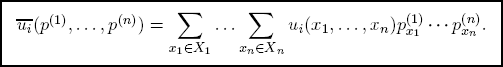
(2) (p) is the expected value of ui relative to the joint probability distribution p = (p(i) i ∈ N) of the players.
The n-person game  is the randomization of the matrix game Γ. The expected total utility value is
As Ex. 6.1 shows, a (non-randomized) matrix game Γ does not necessarily have equilibria. Notice, on the other hand, that the coordinate product function

is continuous and linear in each variable. Each utility function of the randomized game is a linear combination of such functions and, therefore, also continuous and linear in each variable.
Since linear functions are both concave and convex and the state set

of is convex and compact, we conclude:
THEOREM 6.1 (NASH [30]). The randomization  of an n-person matrix game Γ admits both a gain and a cost equilibrium.
REMARK 6.2. An equilibrium of a randomized matrix game is also known as a NASH1 equilibrium.
4.Traffic flows
A fundamental model for the analysis of flows in traffic networks goes back to WARDROP [45]. Let us look at a discrete version2 of it. It is based on a graph G = (V, E) with a (finite) set V of nodes and set E of (directed) edges e between nodes,

representing directed connections from nodes to other nodes. The model assumes:
| (W) | There is a set N of players. A player i ∈ N wants to travel along a path in G from a starting point si to a destination ti and has a set  i of paths to choose from. i of paths to choose from. |
Game-theoretically speaking, a strategic action s of player i ∈ N means a particular choice of a path P ∈  i. Let us identify a path P ∈ i with its incidence vector in ℝE with the components

The joint travel path choice s of the players generates the traffic flow

where  is the number of players that choose path P in s. The component
  of xs is the amount of traffic on edge e caused by the choice s.
We assume that a traffic flow x produces congestion costs c(xe) along the edges e and hence results in the total congestion cost

across all edges. An individual player i has the congestion cost just along its chosen path P:
If we associate with the flow x the potential of aggregated costs

we find that player i’s congestion cost along path P in x equals the marginal potential:

It follows that the players in the WARDROP traffic model play an n-person potential game on the finite set of possible traffic flows.
x ∈ is said to be a NASH flow if no player i can improve its congestion cost by switching from the current path P ∈ i to the use of another path Q ∈ i. In other words, the NASH flows are the cost equilibrium flows. Since the potential function Φ is defined on a finite set, we conclude
•The WARDROP traffic flow model admits a NASH flow.
BRAESS’ paradox. If one assumes that traffic in the WARDROP model eventually settles in a NASH flow, i.e., that the traffic flow evolves toward a congestion cost equilibrium, the well-known observation of BRAESS [6] is counter-intuitive:
| (B) | It can happen that a reduction of the congestion along a particular connection increases(!) the total congestion cost. |
As an example of BRAESS’ paradox, consider the network G = (V, E) with

Assume that the cost functions on the edges are

and that there are four network users, which choose individual paths from the starting point s to the destination t and want to minimize their individual travel times.
Because of the high congestion cost, no user will travel along (r, q). As a consequence, a NASH flow will have two users of path P = (s → r → t) while the other two users would travel along 
The overall cost is:

If road improvement measures are taken to reduce the congestion on (r, q) to  = 0, a user of path P can lower its current cost C(P) = 6 to C(Q) = 5 by switching to the path

The resulting traffic flow, however, causes a higher overall cost:

_____________________________
1 J.F. NASH (1928–2015).