2. Conceptual landscape models
3. Key components of landscape pattern
4. Landscape pattern and biodiversity: Concluding remarks
The amount and spatial arrangement of different types of land cover are major drivers of terrestrial biodiversity. Conceptual landscape models provide the terminology needed to analyze the effects of landscape pattern on biodiversity. Conceptual landscape models vary in their degree of complexity and realism. In increasing order of complexity, conceptual landscape models include the island model, the patch-corridor-matrix model, the variegated landscape model, the hierarchical patch dynamics model, and species-specific gradient models. Less complex models are easier to communicate than complex models, but they may oversimplify the relationship between landscape pattern and biodiversity (especially in highly heterogeneous landscapes). Key components of landscape pattern that have an important effect on biodiversity include patches of native vegetation, the nature of land use outside these patches, the connectedness of patches and ecological processes (connectivity), and the variability in land cover types (heterogeneity). Landscapes with (1) large areas of native vegetation, (2) areas outside patches that are similar in structure to native vegetation, and (3) high landscape heterogeneity are likely to support a high level of biodiversity.
biodiversity. The diversity of genes, species, communities, and ecosystems, including their interactions
conceptual landscape model. A theoretical framework that provides the terminology needed to communicate and analyze how organisms are distributed through space
connectivity. The connectedness of habitat, land cover, or ecological processes from one location to another or throughout an entire landscape
landscape. A human-defined area, typically ranging in size from about 1 km2 to about 1000 km2
landscape heterogeneity. The variability in land cover types within a given landscape
landscape pattern. The combination of land cover types and their spatial arrangement in a landscape
matrix. The dominant and most extensive patch type in a landscape, which exerts a major influence on ecosystem processes
patch. A relatively homogeneous area within a landscape that differs markedly from its surroundings
Life is not distributed uniformly across the surface of the planet. In terrestrial systems, several biophysical variables such as nutrient availability, radiation, and water availability are fundamental influences on where different organisms occur (see chapter IV.1). In addition, in a given area, the types of land cover present and where they occur have a major influence on how biodiversity is distributed through space. This chapter summarizes several conceptual models that are commonly used to help us think about landscapes. These conceptual models facilitate an understanding of the relationship between key components of “landscape pattern” and biodiversity.
The effect of landscape pattern on biodiversity can be analyzed and communicated in many different ways. Implicitly or explicitly, ecologists and nonecologists alike rely on conceptual models that summarize the most important features in a given landscape. Do we need to know where there are trees? Or what the density of buildings is? Or where the warmest areas are that are suitable basking sites for a particular reptile species? Different features of landscapes will be most important for different purposes, and therefore, different conceptual models of landscapes may be required.
A conceptual landscape model can be defined as a theoretical framework that provides the terminology needed to communicate and analyze how organisms are distributed through space. Typically, a conceptual landscape model also can be used to draw a picture of the most important features in a given landscape, that is, to visualize landscape pattern.
There are many different conceptual landscape models, and different people may perceive the same landscape in quite different ways. However, some general conceptual models and descriptions of landscapes and landscape pattern are broadly agreed on and are used by many ecologists. These conceptual models simplify the complexity of landscape patterns. This simplification is useful because it enables meaningful communication, provides a common terminology, and focuses people’s attention on particular features within a landscape. A potential disadvantage of any particular simplification is that important aspects of complexity may be overlooked. In this regard, conceptual landscape models are no different from many other models that face a trade-off between useful simplicity and undesirable oversimplification.
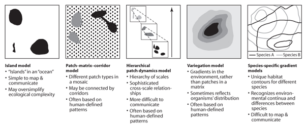
Five conceptual landscape models are outlined in the remainder of this section: (1) the island model, (2) the patch-corridor-matrix model, (3) the hierarchical patch dynamics model, (4) the variegated landscape model, and (5) a suite of species-specific gradient or continuum models. The first two models are widely used, whereas the last three are applied less commonly, although they can be extremely useful.
The island model originates from the equilibrium theory of island biogeography, which was developed to explain patterns in species richness on islands surrounded by ocean (MacArthur and Wilson, 1967; see also chapter IV.3). As a conceptual model for terrestrial landscapes, the island model is based on the analogy of hospitable islands within an inhospitable ocean. Thus, the island model provides a black-and-white view of landscapes—every point in the landscape is classified to be either part of an island or part of the inhospitable surrounds (figure 1). What constitutes an island depends on the purpose for which the model is used. For example, islands might be forests, whereas all other land cover might be considered “ocean”; or islands might be areas of suitable habitat for a species of interest, in which case what constitutes an island depends on the species and its habitat requirements. For a rock fern, rocky outcrops might be suitable islands, whereas tree-cavity-dependent mammals may find suitable habitat only in islands of old-growth forest. The island model is very simple. This attractive simplicity, combined with the broad impact of island biogeography theory, means that it has been very influential. Important insights about what constitute suitable islands or patches have arisen from the island model (see below). However, often the island model can be too simple if considered on its own. Land cover often changes more continuously than is assumed by the island model, and what is an appropriate island for one species may be inappropriate “ocean” for another.
Figure 1. Schematic overview of alternative conceptual landscape models, including a short summary of their key features, strengths, and limitations.
The patch-corridor-matrix model is an extension of the island model. Patches in this model are broadly equivalent to islands, and the matrix is broadly equivalent to the ocean in the island model (see Glossary above). Corridors, the third landscape element, are linear features that connect the patches. The patch-corridor-matrix model is closely associated with a mosaic view of landscapes (figure 1). A mosaic view does not necessarily assume that all patches are equal but may explicitly distinguish among a number of different patch types. These patch types are typically based on human-defined attributes rather than the habitat of a particular species. For example, three patch types might be deciduous forest patches, evergreen forest patches, and mixed forest patches, and all of these might be embedded within a matrix of agricultural land. In this example, linear connections of vegetation between forest patches would be considered corridors. The patch-corridor-matrix model has several important advantages over the island model. First, it recognizes that the matrix plays several important roles in addition to isolating the patches (see below). Second, it acknowledges that corridors fulfill an important connectivity function. Third, it recognizes the role of landscape heterogeneity by considering landscape mosaics composed of various different patch types. The main limitation of the patch-corridor-matrix model is that it is usually based on a human perception of landscapes in which humans define where patches start and end and what the appropriate patch types are. This can be problematic because some organisms perceive their environment in a very different way from humans. For example, the spatial scale relevant to a beetle is much smaller than the scale at which the patch-corridor-matrix model is typically applied. Similarly, some plants and animals may respond strongly to variables that are not easily seen by humans; for example, some plants might be restricted to locations with high fertility, and some cold-blooded animals (or ectotherms) might respond strongly to subtle variations in temperature.
The hierarchical patch dynamics model is similar to the patch-corridor-matrix model in that it also recognizes landscape mosaics. However, it is more complex because it recognizes spatial hierarchies (Wu and Loucks, 1995). That is, it recognizes that patchiness in a given landscape does not occur at only one spatial scale, but, rather, different levels of patchiness are apparent at different scales (figure 1). At a coarse scale, for example, islands of trees might be patchily distributed through a landscape, whereas at a much finer scale, different clumps of grass might be considered as individually recognizable small patches. Hierarchy theory also provides an explicit link between different scales and how they influence one another. In particular, the ecological dynamics at coarse spatial scales is seen as a constraint or context on the ecological dynamics that occurs at finer scales. For example, individual trees in a forest might die when they reach an old age, but if the larger-scale context is continuous forest, it is highly likely that new trees are able to regenerate to replace such dead trees. Thus, the hierarchical patch dynamics model can be applied, for example, to explain the population dynamics of particular species in a given landscape (see chapter IV.3). Although the explicit recognition of spatial dynamics is a key strength of the hierarchical patch dynamics model, its level of complexity means that it is not as easily applied as the simpler island or patch-corridor-matrix models.
The landscape models discussed so far all assume that spatial discontinuities, and therefore patches, can be defined in landscapes. Although this is sometimes the case, in other cases it is unclear where patch boundaries should be drawn. The absence of obvious spatial discontinuities led to the development of the variegated landscape model. This model recognizes that land cover may change continuously through space—for example, dense tree cover may gradually blend into widely scattered trees, and these may increasingly blend into open grassland (figure 1). Superimposing islands onto a landscape with gradual changes can be a serious oversimplification. For example, many species may not be strictly dependent on predefined islands of forest but may use the continuous gradient from forest to grassland to different extents. The variegated landscape model provides a viable alternative to patch-based models in situations where it can be shown that organisms respond continuously along a gradient of landscape change. Its main contribution—to highlight that some patterns cannot easily be translated into a patchy view of the world—is important at a conceptual level because it questions one of the fundamental assumptions made by mosaic- or patch-based landscape models.
To different extents, the models discussed above rely on a classification of landscape pattern that can be readily perceived by people. What resonates with people, however, may not be a good way to characterize a landscape from the perspective of other species. Similarly, how one organism perceives a given landscape may be vastly different from how another perceives it. In fact, no two species are likely to perceive a given landscape in the same way. Indeed, even different humans perceive the same landscape in different ways. For this reason, a different suite of landscape models attempts to see landscapes from the perspective of a given organism of interest. Rather than predefining land cover as a mosaic or as a continuum of predefined land cover, species-specific gradient models start with a particular organism and then attempt to quantify how suitable a given point in the landscape is for that organism. This quantification can occur either empirically (using observed data) or by considering a series of key requirements of the organism, such as its needs for nutrients, shelter, space, climatic conditions, and the abundance of mutualists, competitors, and predators. Such species-specific gradient models can be visualized by drawing maps of where a given species of interest is most and least likely to occur (figure 1). Two key strengths of these models are that (1) they do not assume that the same landscape classification will necessarily work for different species, and (2) they encourage their users to think about fundamental ecological processes shaping the distribution of a species. A weakness of species-specific gradient models is that many different visualizations of a given landscape would be needed to reflect the needs of many different species. Typically, this is too complicated to be feasible, except in cases where only one or few species are targeted. In addition, such models are more difficult to communicate and are not easily depicted in Geographical Information Systems and maps. Thus, as for the variegated landscape model, the most useful contribution of species-specific gradient models may be at a conceptual level: they encourage their users to question key assumptions that are implicit in some of the other landscape models.
The different landscape models have different strengths and weaknesses and are suitable for different purposes. None of them is inherently right or wrong. To reduce the risk of oversimplifying complex ecological systems, it can be useful to think about a given scientific or management problem in more than one way, that is, to apply more than one landscape model and think about the contrasting insights obtained. Key features of the different landscape models are summarized in figure 1.
Although different landscape models will highlight different components of a landscape pattern, the important influence of some particular landscape features on biodiversity is now widely accepted (reviewed by Lindenmayer and Fischer, 2006). Four such features are discussed below: (1) patches of native vegetation, (2) modified land surrounding these patches, (3) corridors and other features that enhance connectivity, and (4) landscape heterogeneity.
The benefit of patches of native vegetation for biodiversity has long been recognized. More specifically, it is widely accepted that, other things being equal (which they may not always be), large patches of native vegetation support more species than smaller patches. Several plausible reasons that are not mutually exclusive have been proposed to explain this pattern:
Similar in importance to patch size at the local scale is the total amount of native vegetation in any given landscape, which is positively related to the overall level of biodiversity at the landscape scale. Species are typically lost from a given landscape with any substantial loss of native vegetation, and the more native vegetation is lost, the more species become locally extinct. At particularly low levels of native vegetation cover, such as when native vegetation covers less than 30% of the landscape (Andrén, 1994), there is some evidence that species loss accelerates beyond the rate of loss observed as cover declines at higher levels of native vegetation.
An additional variable influencing how patches of native vegetation affect biodiversity is how these patches are distributed through space. Broadly speaking, for any given total amount of native vegetation cover, two extreme types of spatial arrangement are possible: (1) many small patches can be dispersed through the landscape, or (2) few large patches can be aggregated near one another. This has led to the “SLOSS” (single large or several small) debate (see chapter IV.3 under “habitat fragmentation”). Evidence to date on which arrangement supports more biodiversity is not clear-cut. In part, which spatial arrangement is better depends on the species of interest. A species that requires large patches would benefit from aggregated large patches, whereas dispersed small patches may be of little value to them. Other species, especially mobile ones such as some birds or bats, may be able to survive in landscapes with many dispersed small patches, partly because they can easily move between patches and thereby access different resources from different patches. The body size of organisms is also important in this context—what constitutes a small patch for a large mammal (such as an elephant) may be perceived as a very large patch by a small reptile (such as a skink).
The amount of species turnover through a landscape also influences whether many dispersed small patches support more biodiversity than few large patches. Where species composition changes substantially through space, many small patches scattered throughout a landscape may effectively sample a higher diversity of species than few large patches aggregated in only part of the landscape, provided, of course, that there are enough species that are not entirely restricted to large patches.
In the early stages of conservation ecology, interest was mostly in patches of native vegetation and their contribution to biodiversity, with little attention paid to the role of the surrounding environment. Areas of nonnative vegetation were often not considered at all, and sometimes they were explicitly considered worthless or even hostile.
Partly because many landscapes worldwide are no longer dominated by native vegetation, ecologists were forced to have a closer look at the effects of modified environments on biodiversity. Most ecologists now believe that areas outside patches of native vegetation, especially if they dominate a given landscape, have a fundamental influence on the biodiversity of that landscape.
There are at least three key ways in which areas outside patches are important. First, in areas that are largely cleared of native vegetation, other land uses typically have a dominant effect on a wide range of ecosystem processes. For example, in industrial tree plantations, wind speeds are higher at the edge of cleared stands; and in suburbia, introduced plants and animals often originate from people’s gardens. Such changes in ecosystem processes, in turn, have an important effect throughout a given landscape, affecting biodiversity both within and outside patches of native vegetation.
Second, some elements of biodiversity can survive outside patches of native vegetation. For example, some bird species inhabit suburban gardens, some frog species breed in puddles adjacent to dirt roads, and some large carnivores may find food in farmland or in urban rubbish tips. The presence of native species outside patches of native vegetation does not mean that native vegetation is not important. Rather, it highlights the point that simply discounting human-modified environments as nonhabitat is overly simplistic.
Third, the nature of areas outside patches of native vegetation dictates to a large degree to what extent species can move from one patch of native vegetation to another. Roadside vegetation, for example, can assist the movement of birds between woodland patches in both rural and urban areas. Similarly, at much larger scales, whether species are able to shift their ranges in response to climate change will depend to a large degree on whether they can move through modified environments.
In summary, notwithstanding the importance of native vegetation patches for biodiversity, what happens outside these patches cannot be ignored. In many instances the patches of native vegetation and their surrounds deserve equal attention because both are fundamentally important and interact in significant ways.
In its broadest sense, connectivity is related to how connected biodiversity is between various locations. Although there is general agreement that connectivity is important, there is far less agreement about what its precise definition should be. Some ecologists believe that connectivity is a property of patches, whereas others think it is a property of entire landscapes. Some believe that it applies to individual species, whereas others think it should apply to a broad suite of ecosystem processes. In this section, we first define three types of connectivity that have been suggested, to overcome some of the vagueness in terminology. We then summarize how landscape pattern is related to connectivity.
Structural connectivity occurs when one part of a landscape is physically linked with another part. The most well-known example is wildlife corridors (see above) linking one patch of native vegetation with another patch. A main aim of maintaining or creating this type of structural link is to facilitate the movement of wildlife. Functional connectivity acknowledges that simply having a structural link may not necessarily facilitate movement for all species; that is, a given corridor may not function in the way it was intended to function if the target species does not use it. There are many reasons why some species are reluctant to move through corridors. For example, predation risk may be higher in corridors than in continuous patches of native vegetation, or certain key resources may not be available. Ecological connectivity is a more general term used to describe the connectedness of ecological processes in a given landscape, either abiotic (such as water flows) or biotic (the spread of weeds, or the annual migration of many bird populations).
Landscape pattern affects all three types of connectivity. Typically, having structural links makes it more likely that functional connectivity and ecological connectivity are also achieved. For this reason, corridors can be a useful strategy to enhance connectivity. Some authors warn that corridors may also have undesired consequences; for example, they may facilitate the spread of fire or weeds or introduced predators (Simberloff et al., 1992). Notwithstanding the possibility of negative consequences, in most cases, the positive consequences of corridors outweigh the risk of negative consequences (Noss, 1987).
Two other features of landscape pattern can also facilitate connectivity. The first is stepping stones. Stepping stones are small patches of vegetation scattered throughout a landscape. Some organisms can use them to move through a landscape. Second, the nature of the “matrix” itself—the dominant land cover type— has a large effect on connectivity. In general, connectivity is likely to be higher if the matrix is similar in structure to native vegetation.
Organisms differ in their habitat requirements. It follows that at a landscape scale, spatial variability in the properties of land—landscape heterogeneity— may be beneficial for biodiversity. Some agricultural landscapes can support high biodiversity because of their heterogeneity. Traditionally managed agricultural landscapes in Europe are good examples. In these landscapes, often a variety of crops is grown in relatively small fields, forest patches are scattered throughout the landscape, and field margins contain seminatural shrubland or specifically established hedgerows. Different species can use different parts of this diverse landscape mosaic, and landscape heterogeneity has been identified as a key variable enhancing biodiversity in European agricultural landscapes (Benton et al., 2003).
Landscape heterogeneity also may result from more subtle changes through space rather than abrupt changes in land cover. Gradual changes in the biophysical properties of landscapes are common in both natural and human-modified landscapes. For example, topography has a major effect on water flows and the distribution of nutrients in a landscape, and the orientation of a given slope can make it warmer and drier or cooler and wetter. Biophysical gradients have long been recognized by plant ecologists as having a major effect on species’ distributions: variables such as temperature, radiation, water, and nutrient availability are particularly important for plants. Animals also may be affected by ecological gradients, although these may be related to different life history requirements such as the availability of sufficient food, space, and shelter. As with heterogeneity in land cover types, the presence of strong ecological gradients within a given landscape can be related to high levels of biodiversity at the landscape scale.
Landscapes can be conceptualized in many different ways. Some conceptual landscape models are simple (e.g., the island model), whereas others are complex (e.g., the hierarchical patch dynamics model). Similarly, some conceptual landscape models are well known, whereas others are less widely known, although they can provide useful insights (e.g., the variegated landscape model). Often, complementary insights can be gained by conceptualizing landscapes in several different ways. For example, the island model may highlight the importance of large patches of native vegetation, whereas species-specific gradient models draw attention to the value of landscape heterogeneity because what may be suitable habitat for one species may not be suitable for another species. Which landscape model is most appropriate in a given situation depends on the particular objectives of the study or management problem in question.
Table 1. Overview of important components of landscape pattern and their effects on biodiversity
Component of landscape pattern |
Effect on biodiversity |
Patches of native vegetation |
|
Areas outside patches of native vegetation |
|
Connectivity |
|
Landscape heterogeneity |
|
Irrespective of the conceptual landscape model used, many factors determine how landscape pattern influences biodiversity (summarized in table 1). Typically, different landscape patterns will support different elements of biodiversity. In general, landscapes with a broad mix of landscape components and a large amount of native vegetation are likely to support high levels of biodiversity.
Andrén, H. 1994. Effects of habitat fragmentation on birds and mammals in landscapes with different proportions of suitable habitat—a review. Oikos 71: 355–366.
Bennett, A. F., J. Q. Radford, and A. Haslem. 2006. Properties of land mosaics: Implications for nature conservation in agricultural environments. Biological Conservation 133: 250–264.
Benton, T. G., J. A. Vickery, and J. D. Wilson. 2003. Farmland biodiversity: Is habitat heterogeneity the key? Trends in Ecology and Evolution 18: 182–188.
Fahrig, Lenore. 2003. Effects of habitat fragmentation on biodiversity. Annual Review of Ecology, Evolution and Systematics 34: 487–515.
Forman, Richard T. T. 1995. Land Mosaics: The Ecology of Landscapes and Regions. New York: Cambridge University Press.
Haila, Yrjö. 2002. A conceptual genealogy of fragmentation research: From island biogeography to landscape ecology. Ecological Applications 12: 321–334.
Lindenmayer, David B., and Joern Fischer. 2006. Habitat Fragmentation and Landscape Change. Washington, DC: Island Press.
MacArthur, Robert H., and Edward O. Wilson. 1967. The Theory of Island Biogeography. Princeton, NJ: Princeton University Press.
McIntyre, Sue, and Richard Hobbs. 1999. A framework for conceptualizing human effects on landscapes and its relevance to management and research models. Conservation Biology 13: 1282–1292.
Noss, Reed F. 1987. Corridors in real landscapes: A reply to Simberloff and Cox. Conservation Biology 1: 159–164.
Simberloff, D. A., J. A. Farr, J. Cox, and D. W. Mehlman. 1992. Movement corridors: Conservation bargains or poor investments? Conservation Biology 6: 493–504.
Wu, Jianguo, and Orie L. Loucks. 1995. From balance of nature to hierarchical patch dynamics: A paradigm shift in ecology. The Quarterly Review of Biology 70: 439–466.