2. Dynamics of geographic populations
3. Patterns in genetic variation and adaptation
4. Synthesis: How spatial patterns in species diversity are generated and maintained
5. Empirical sampling protocols
6. Species abundance and relative abundance distributions
8. Abundance–distribution relationships
9. Nested subsets community pattern
10. Species diversity along environmental gradients
11. Understanding species diversity
Spatial patterns of species diversity have intrigued ecologists since European natural historians discovered that the flora and fauna of the world varied dramatically across the face of the Earth. It is only within the last few decades that a clear understanding of the processes underlying these patterns has arisen. Variation in the number of species found across space depends on several interacting sets of processes. The first set of processes affect the physical and chemical properties of the hydrosphere, atmosphere, and lithosphere. The second set of processes comprises the demographic responses of individual organisms interacting with their physical and biological environment summed up within geographic populations of different species. The final set of processes are the long-term adaptive responses of populations as natural selection shapes gene pools of different species over evolutionary time. The complex interactions of these sets of factors occur across a wide range of spatial and temporal scales, making it difficult to isolate simple explanations for data collected at single spatial and/or temporal scales.
In what follows, I provide an outline for how the three sets of processes work together to set the broad patterns of species diversity seen across geographic space. Here I focus on terrestrial patterns, although a similar argument applies to marine patterns of species diversity. After outlining the processes underlying species diversity variation, I show how different methods of sampling species diversity across geographic space produce the variety of patterns documented by ecologists and biogeographers.
adaptive syndrome. The suite of morphological, physiological, and behavioral characters that determine an organism’s ability to survive and reproduce
α diversity. The species diversity of a locally sampled site
β diversity. The turnover in species diversity among different sites within a landscape, generally referring to sites that share the same metacommunity
γ diversity. Turnover in species diversity among different metacommunities
geographic population. All viable populations of a species found within the species’ geographic range
geographic range. The spatial region that includes all viable populations of a species
metacommunity. For any given local community, the assemblage of all geographic populations that contribute immigrants to the community
metapopulation. A group of local populations linked together by dispersal
species diversity. The number and relative abundances of species within a specified geographic region, often divided into α, β, and γ diversity
viable population. Any population that can persist through time by a combination of local recruitment and immigration
Spatial patterns of species diversity result from the interplay of biology with large-scale patterns in the physical properties of the Earth. For a complete description of diversity patterns, then, it is necessary to describe the dynamics of the physical system that comprises the thin layer of materials covering the Earth. Several important sources of energy drive the geophysical environment. Of these, the most important from the perspective of living systems is the sun. Energy from the sun not reflected back into space is absorbed by the surface of the Earth and the atmosphere. The absorbed energy heats air masses in the atmosphere, causing large vertical circulation patterns that distribute water in the atmosphere unevenly across the surface of the Earth. These movements result in broad patterns of climate with latitude, with wet tropical climates near the equator, bands of arid climates at approximately 30° latitude, and wetter temperate climates at 60° latitude (see chapter IV.7 for a more detailed account).
Modifications of the general patterns of heat distribution across the face of the Earth and the consequent movements of air masses across its surface incorporate a number of different processes. The rotational energy of the Earth modifies these general patterns, particularly near coastal regions. The tilt of the Earth results in seasonal patterns in climate as the Earth travels around the sun. Topographic features of the Earth’s crust deflect movements of air masses upward, changing nearby patterns of precipitation. Gravitational energy from the moon causes large movements of water masses in the oceans, resulting in tidal patterns along continental margins. These factors combined result in heterogeneous patterns in the spatial distribution of water, and of its different states (i.e., gas, liquid, solid). The tremendous variability in the distribution of water determines to a large degree the distribution of life on the planet.
The crust of cooled rocks on the Earth’s surface is not a static entity. The lithosphere is a dynamic system driven primarily by energy derived from the Earth’s molten core. Over long spans of time (millions of years), movements of pieces of the crust redistribute continental land masses and change the configurations of the oceans. As land masses shift, so do many of the factors that determine climate. Hence, there is a continual shifting in the distribution of water across the Earth and, consequently, of living systems.
Because all living systems (with a few minor exceptions) are based on energy captured by photosynthesis, variation in the amount of solar radiation across the surface of the Earth also affects the distribution of primary production. This variation in solar energy for photosynthesis interacts with complex patterns of water distribution to form the major biomes recognized by ecologists. Additional variations in the physical conditions of the Earth’s surface are imposed at a variety of scales by topography, geology, and a variety of disturbances.
Patterns of species diversity are responses of living systems to the complex geophysical variation described in the previous section. These responses involve a wide variety of phenomena that occur across different expanses of space and time. The processes involved in generating these responses can be divided into ecological and evolutionary processes, but this division is arbitrary, for ecological and evolutionary phenomena are closely linked and constitute a single system that integrates living and nonliving components into a single, highly complex hierarchy. In this section I focus on the fundamental ecological processes that underlie species diversity patterns.
At the smallest spatial scale, individual organisms respond to environmental variation through a variety of physiological, morphological, and behavioral adaptations. By definition, these adaptations are fixed within an organism, although they may involve changes in the way an organism interacts with the environment throughout its lifetime. The fundamental importance of these adaptations with respect to species diversity patterns is that they determine the survival and reproduction of individual organisms as they interact with localized environmental conditions. Although there are many complications and variations on patterns of organismal interactions, the fundamental consequence of these interactions is that they determine the rate of change and persistence of populations of organisms belonging to the same species. Species in this sense consist of organisms that share a genetic cohesiveness that maintains the system of adaptations among all organisms belonging to the species. Many times, this means that members of the same species exchange genes through various types of reproductive activities.
Populations are often arbitrarily divided into local concentrations of individuals in space. Within a population, organisms give birth and die in response to local environmental conditions. Over time, the number of organisms in the population changes as a consequence of these organismal patterns. Most populations are not closed systems with respect to the organisms that comprise them. Organisms born elsewhere enter the population, and other organisms leave the population and move elsewhere. The rate of local population change is determined by the rates of birth, death, immigration, and emigration.
Over larger expanses of space, organisms are almost never randomly or uniformly distributed but clump into local concentrations that experience unique sets of environmental conditions. Often these localized clusters are separated sufficiently to be treated as distinct populations that are linked to one another by dispersal. Systems of local populations linked together by dispersal are called metapopulations. The boundaries of a metapopulation are rarely explicitly known, and across geographic space, there may be many metapopulations for a single species. Metapopulation dynamics has been described in two different but related ways. First, equations that describe changes in abundance within local populations that include both birth–death and immigration–emigration dynamics are used to describe spatial patterns in the dynamics of the collective metapopulation. Second, extinction–colonization processes are used to describe the spatial pattern of occupancy of local habitable “patches” within metapopulation boundaries (see chapter IV.3 for further discussion of metapopulation dynamics).
When we consider the collective population across the range of most species, we see a distinct pattern in which there are relatively few locations with large concentrations of abundance and many locations with fewer individuals. This pattern may be generated by two different patterns within local populations. First, local populations may have higher densities near abundance peaks and lower densities away from those peaks. Second, density may be relatively constant across the geographic range, but distances among local populations may be larger in many regions of the range. When averaged across space, this pattern would produce an uneven distribution of abundance across the range. Regions of high abundance often cluster close to the geographic center of the range. In some species, there may be a single region of high abundance, whereas in others there may be several regions. Differentiating between these two possibilities is difficult in practice because of the discontinuous nature of ecological conditions experienced by individuals of different species.
The abundance patterns just described are generated by spatial variation in demographic processes across the range of a species. It appears that for many species, regions of high abundance are characterized by high per capita maximum growth rates coupled with lower per capita intraspecific competition. Conversely, low-abundance regions have low maximum per capita growth rates and higher intensities of intraspecific competition. It is also possible in some cases to model the role of dispersal in maintaining these patterns. When this is done, dispersal seems to be a crucial part of local demography when there are large changes in geographic ranges, e.g., during an invasion by a species into a new geographic region. Estimation of these patterns is made more difficult by the fact that there is often a large degree of environmental variation. Additionally, many methods of estimating abundance include measurement error, which can produce poor estimates of population rates if not included in estimation procedures.
Spatial patterns in demography are linked to the conditions individuals experience in their local environments by suites of behavioral, physiological, and morphological traits, which together can be termed the “adaptive syndrome” of a species. When most of the individuals in a population possess traits that function well in a particular environment, then the fitness of individuals in that population is high, leading to a sustainable population. Conversely, when few individuals in a local population have traits that allow them to function in the local environment, the population itself will be less stable and often may be a “sink” population maintained by immigrants coming from populations with high per capita fitness. To the degree that per capita fitness is correlated with abundance, population abundance will follow spatial patterns in fitness. The fundamental insight is this: large-scale spatial patterns in the distribution of abundance are maintained by spatial variation in demographic responses of local populations to environmental conditions.
Notice that it is not necessary to invoke the concept of a “niche” in this discussion. The adaptive syndrome concept is not equivalent to what many ecologists refer to as a niche. Whereas the idea of an ecological niche invokes references to local interactions among species or some idealized hypervolume describing the ecological “needs” of a species, the necessary concepts to describe geographic distributions are not based on such vague notions. Instead, what are needed are adequate descriptions of the demographic mechanisms that result from the demographic responses of individual organisms within a population to the conditions they experience in the environment.
The traits that organisms employ to obtain sufficient resources for survival and reproduction play a crucial role in shaping the demographic responses of local populations to environmental conditions. These traits are the result of a long history of natural selection and other evolutionary processes shaping the current genetic makeup of each local population. The same patterns of immigration and emigration responsible for the dynamics of geographic populations spread and mix genetic variation within and among local populations. Natural selection demographically corresponds to increased mortality and/or reduced fecundity in at least some of a local population. Gene flow from populations in more productive environments can dilute genetic changes that might be more adaptive in local populations. Conversely, lower rates of gene flow to isolated populations may allow changes in genetic structure in response to selection.
The complex counterplay of migration and selection ultimately leads to suites of ecological characteristics within species (the adaptive syndrome defined previously) that link environmental conditions to demographic responses in ecological time. The adaptive syndrome of a species and the environmental context in which it is expressed together constitute what is sometimes called the “niche” of a species, although this term often has conflicting and ambiguous meanings in the ecological literature. When thinking about patterns of species diversity, it is preferable to think of the adaptive syndrome of a species as a distinct concept because it allows comparisons among species in their potential to respond to gradients of environmental conditions in space and time.
The fundamental concept behind understanding large-scale patterns of species diversity is the idea of a metacommunity. Defining what a metacommunity is turns out to be quite difficult. The model described in what follows incorporates most of the insights into this problem represented in the literature. A metacommunity is the collection of all species of a given trophic group that contribute populations of individuals within a specified region. For example, the metacommunity for the plants found in Yellowstone National Park, in North America, will include the geographic ranges of all species found there. Depending on the size of the geographic region involved, most species will have at least some populations outside of the region. Only when the region considered reaches the size of a continent or the degree of isolation of a remote island will most species’ geographic ranges be contained within the region. In general, then, the metacommunity will cover a larger spatial region, approaching the size of a continent for some groups, than the particular community for which it serves as a source of species. The idea of a metacommunity includes what is often termed a “species pool.” In some senses, a metacommunity represents the “γ diversity” of the geographic region for which it serves as the species pool.
Many spatial patterns in species diversity are based on comparisons of different geographic regions along an environmental gradient. Defining the metacommunity for a set of regions may become problematic because each region will have a different set of species that would meet the criterion proposed in the previous paragraph. Each separate region, such as regions defined by latitudinal bands, has different γ diversities, making comparisons among them complicated.
Recently, the importance of the size and shape of the geographic gradient has been shown to contribute to patterns of species diversity. The “mid-domain effect” simply states that the larger the region across which species diversity is measured, the larger the accumulation of species will be. Thus, if an environmental gradient is embedded in a geographic region that varies in size along the gradient, the effects of the gradient on species diversity will be confounded with the effects of area. This effect of the size and shape of a geographic region was first identified in studies of species diversity along latitudinal gradients. For example, species diversity of birds decreases with decreasing latitude in southeastern North America and the Florida peninsula, where the constraining effects of geographic area contribute to a reversal of the general pattern of increasing species diversity with decreasing latitude elsewhere on the continent.
Given the complications discussed above, spatial patterns of species diversity all arise from the same basic mechanism. Species that comprise the metacommunity for a particular geographic region provide the source of individuals that potentially have access to a local community. These immigrants can enter a local community under a variety of conditions. If all individuals in the metacommunity are ecologically identical regardless of species (i.e., there is ecological symmetry among species), then a stochastic process that depends on local birth–death processes coupled with immigration drives local community dynamics. When immigration is absent, the process leads to fixation of a single species in the local community. With the addition of immigration, the process will eventually equilibrate relative abundances of species in the local community with corresponding relative abundances in the metacommunity. This model of community, known as the neutral model, emphasizes the importance of dispersal processes in maintaining local species diversity.
The neutral model is often thought to be unrealistic in its assumption of ecological symmetry among species. The effect of breaking the symmetry assumption is more difficult to model dynamically, but the basic effects of ecological asymmetry on local communities are straightforward. The fundamental result is that when asymmetry exists, the environment in which a local community exists acts as a “filter” on both local demographics and immigration. Generally, this filtering effect maintains rare species in local communities by preventing extinction and encouraging immigration. The filter effect of the local environment is analogous to “natural selection” in the population genetics models. In addition, some of the filtering within a community is caused by interspecific competition. The effect of such competition is to restrict species spatially to patches in the local community where they are competitively superior. If there are insufficient “refuges” for a species, then competition may act as a strong filter, permitting only certain combinations of species.
Given the general stochastic model that couples dispersal and local environmental filtering into a community dynamic, communities can be compared among different local sites and across time. Each local community has a resistance to change based on the adaptive syndrome of each species and the nature of the environmental conditions. This “community inertia” represents a steady state that will persist until some environmental change is experienced. The response of a local community to environmental change is not instantaneous but requires a certain amount of time over which local demographics and patterns of immigration shift in response to changing conditions.
When local communities are compared across space, the resulting patterns are produced both by differences in local ecological conditions and by differences among the metacommunities that are sources of immigrants. The expectation of community inertia across space implies that there will be spatial autocorrelation among communities that declines with distance. This distance effect corresponds to the concept of β diversity. Note that β diversity, in this sense, will respond to both metacommunity properties and variation in local ecological conditions across space. Disentangling the contributions of these two factors remains a major challenge to understanding why species diversity varies across geographic space.
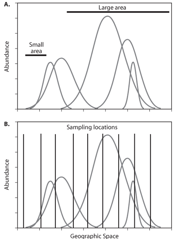
Given the general approach described above, we are now ready to examine empirical patterns that arise when researchers measure species diversity in the field. Most empirical patterns of species diversity are obtained under three general sampling regimes. The first is area sampling. Area sampling occurs when a geographic region is divided into areas of different sizes (figure 1A). Most often, the total number of species is counted within regions, but occasionally abundances or densities for each species within the region are available. The quintessential area-sampling regimen of this sort is counts of species number on oceanic islands of various sizes and degrees of isolation. Habitat islands are another variation on area sampling. Area sampling is useful when there are clear demarcations of areas into different ecological units. In some regions, there are no clearly established or easily identifiable ecological boundaries. In such situations, a modification of area sampling consists of nesting smaller sample areas within larger ones. This nested-area sampling approach (figure 1A) produces similar results to area sampling, but there is a component of spatial autocorrelation because of the accumulating total species richness from smaller, nested areas into larger areas. It is possible to reduce such autocorrelation with an appropriately designed sampling protocol. The final sampling protocol used to assess patterns of species diversity is a point sampling. The salient feature of point sampling is that each “point” represents a relatively small area of sampling that does not vary in size from location to location (figure 1B). Point sampling is often conducted as part of a transect placed along an environmental gradient. The size of the area actually sampled varies widely, from small plots (measured in square meters) up to regions spanning many square kilometers (i.e., 1° latitude-longitude blocks).
Figure 1. Schematic representation of different sampling protocols for examining spatial patterns of species diversity in space. Species distributions are shown as Gaussian distributions for simplicity. What is necessary, however, is that the geographic range be finite and abundance unevenly distributed within the boundaries. Space is represented as a single dimension, but most patterns are observed in two spatial dimensions. (A) General approach of area sampling. Samples of different sizes are located in space, and all species falling within a given area are counted (and sometimes estimates of abundance are obtained). Islands are a form of area sampling applied to ecosystems that have distinct boundaries where individuals can occur only within the boundaries. Nested-area sampling consists of nesting smaller areas within larger ones. (B) Point sampling. Point samples of the same size (often relatively small compared to the ranges of species) are located in space using some sampling protocol. Species are identified, and sometimes abundance is estimated, within the sampling plots.
There are three basic assumptions about the nature of the metacommunity that are required for the sampling schemes described above to generate empirical patterns. First, the range of each species must be restricted to a part of the geographic region occupied by the metacommunity. This restriction might be a result of environmental filtering, dispersal limitation, or a combination of the two. Second, the ranges of species within the geographic region must vary in size. Although there can be overlap among ranges, both the size and region occupied by each species must vary in a nonuniform manner within the geographic region. Finally, for some patterns, it is necessary that abundances of each species be nonuniformly distributed within the boundary of their geographic range. All of these assumptions are consistent with the description provided above of the demography underlying geographic distributions of species.
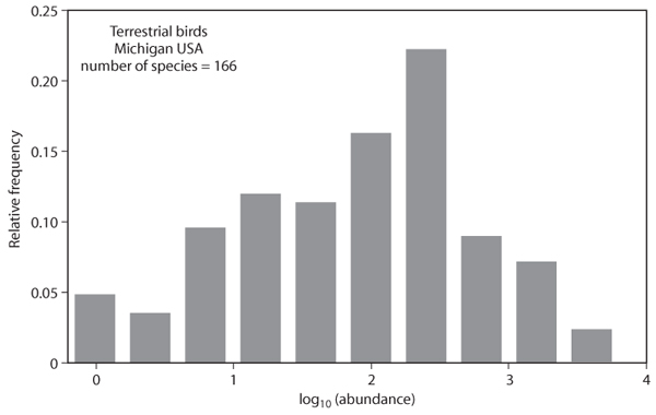
The most fundamental result pertaining to sampling communities within a larger metacommunity is that there are few common species and many rare species (figure 2). This pattern is nearly universal across all communities regardless of environment or taxonomic composition. Furthermore, aggregating communities in space or time does not change the pattern, although the position of individual species may change. The pattern occurs in metacommunities, geographic regions, and entire continents.
The basic assumptions described above have, as a direct consequence, this uneven distribution of abundance. Because a species cannot be found everywhere, and its abundance is unevenly distributed within its geographic range, there must inevitably be some species at a geographic location that have adaptations that more closely match environmental conditions than most of the species in the community. Other species persist in the community by finding refuges from superior competitors, using resources that are marginal to other species, or by persisting as a sink population maintained by immigration from a larger metapopulation.
Figure 2. Distribution of abundances of 166 species of terrestrial birds found within Michigan. Data were obtained from the North American Breeding Bird Survey (BBS). Average abundances were calculated from 2000 to 2005 across all BBS routes found in Michigan.
What remains unexplained is the reason why species have different geographic range sizes. Why do the adaptive syndromes of a group of related species result in some species that are able to use a wider range of conditions than others and, hence, that have larger geographic ranges? Although we are far from understanding the answer to this question, the essence of the problem may be the necessary trade-offs that occur during microevolution. Both environments and organisms are complex and capable of change, but in order to persist in some environments, species must compromise their ability to persist in others. This leads to the potential for conflicting selection pressures in different environments. The gene pool of a species has only a limited amount of potential phenotypes that can be generated. Organisms living in environments that allow them to produce the most offspring will contribute more to the reservoir of genetic information than organisms living in other environments. This will tend to dampen out selection occurring in marginal environments via gene flow.
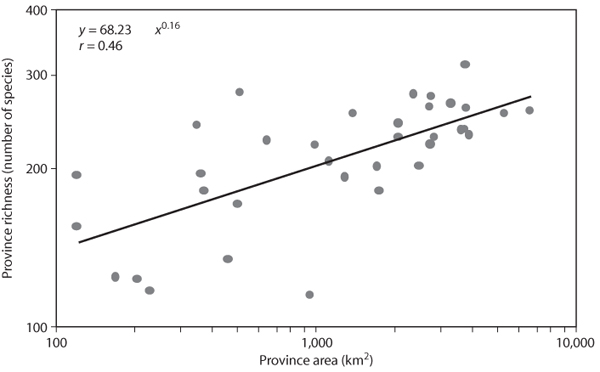
Perhaps one of the best-known of all species diversity patterns is the positive relationship between the size of an area and the number of species found in it (figure 3). This is a direct consequence of area sampling. When an area is located randomly within the ranges of a group of species, the size of that area determines how many rare species will be included in that area. Species may be rare in the region because either they are globally rare or they are at the margin of their geographic range. Smaller areas have a higher probability of not including species with restricted ranges. In other words, area alters the probabilities of species in the metapopulation appearing in local samples. In a completely mixed metacommunity, where all species are equally probable to appear in all samples, the species–area relationship disappears.
Variation in the shape of species–area relationships is related to the degree to which local communities sample the metacommunity. This, in turn, is related to the relative size of the region over which the species–area relationship is being studied. For large regions such as continents, species number increases relatively rapidly with increasing area because most species will not occur over the entire region. As the region of focus becomes smaller, such as samples taken across a biome within a region, the metacommunity being sampled does not contain rare species restricted to ecological conditions not found in the region. The increase in species with increasing area is lower. Isolation of a geographic region also affects the species–area relationship. Isolation has the effect of restricting dispersal of species within the metacommunity, effectively decreasing immigration rates. This will also lower the rate at which species richness increases with area. For example, islands typically have lower slopes for log-log plots of species richness against area than nearby mainlands.
Figure 3. Relationship between number of species and area among 35 ecological provinces recognized by the U.S. National Ecological Unit Hierarchy. Only provinces found within the contiguous United States are reported.
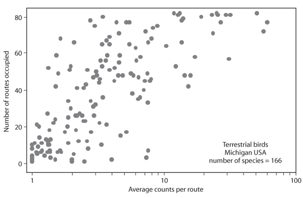
Figure 4. Relationship between distribution (number of routes occupied) and average abundance for 166 species of terrestrial birds found in Michigan.
In a point sampling study, the average abundance of each species increases with the number of points the species occupies (figure 4). This is the result of the nonuniform distribution of abundance within a species’ range and the fact that, if a species shows up more often across sample points, it is more likely that the metacommunity defined for that particular set of samples is located around range abundance centers for that species. There will undoubtedly be variation in the way that each species is distributed within the region, so it is not expected that the correlation between average abundance and distribution will be perfect.
Abundance–distribution relationships can be obtained at many different sampling scales. Within a single landscape, point sampling will produce a positive correlation assuming nonuniform spatial distributions of individuals of different species within the landscape. In such a situation, all samples are assumed to be drawn from the same metacommunity. As the spatial scale of the sampling increases, crossing of ecological boundaries results in some points having different metacommunities. The abundance–distribution relationship in such cases would summarize both variation among points and variation among metapopulations. The likely result of this is to increase the scatter about the abundance–distribution correlation. When the region being measured includes an entire continent, there will be a very large number of metacommunities involved in the abundance–distribution correlation, resulting in a relatively large degree of scatter among different point samples.
Under an area-sampling scenario, larger areas are more likely to contain the rarest species in a metacommunity than smaller areas. This is because species with the smallest ranges have the lowest probability of being included in a randomly located sampling area. As the sampling area increases, the probability of including a species with a small geographic range increases. On average, then, rare species occur only in the largest sampling regions. Conversely, species with the largest geographic ranges have the highest probabilities of being included in a sample of a given size. Smaller sampling areas, on average, will tend to have only the most widespread species found in them.
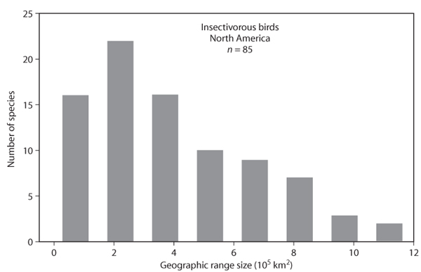
The pattern described in the previous paragraph has been termed the “nested subsets” pattern because the species found in smaller sampling regions are nonrandom subsets of the species found in the largest sampling regions. The crucial assumption required for this pattern to obtain is that there must be a nonuniform distribution of geographic range sizes, with a relatively large number of ranges of small size, coupled with a smaller number of species with large ranges (figure 5).
Because species are not capable of being found everywhere, as one moves across space, the species composition of local communities changes. The turnover in species, or β diversity, follows directly from application of the assumptions made above. There has been a long tradition in ecology and biogeography that seeks to understand this turnover by observing species composition along some identifiable environmental gradient, such as a moisture, elevational, or latitudinal gradient. The patterns observed along such gradients are thought to indicate how the gradient itself affects the loss of some species and the inclusion of others in local communities. To this end, many studies of species diversity along gradients have opted to study patterns across major environmental gradients at geographic scales.
Figure 5. Distribution of geographic range sizes of 85 insectivorous birds found in North America.
Perhaps the most controversial of these types of studies are studies of species diversity along latitudinal gradients. Many environmental conditions change with latitude, as described earlier. Generally, latitudes closer to the equator have warmer and/or wetter climates. If warm, wet climates support higher levels of primary production, it follows that species diversity should be highest in tropical latitudes. Although this is generally true, there are many qualifiers to these patterns. For example, some taxa show distinct patterns of increasing diversity with increasing latitude. Furthermore, continental areas vary strikingly with latitude, implying an overriding influence of continental area on species diversity patterns that are independent of climate. General explanations for latitudinal diversity gradients are difficult to generate and test.
Rather than collecting point samples along a latitudinal gradient, some researchers have attempted to relate species diversity directly to ecologically significant environmental factors that have complex patterns of spatial variation. Many of these studies relate species diversity directly or indirectly to some measure of energy production. For example, many studies have shown that species richness in point samples correlates positively with the rate of evapotranspiration. Evapotranspiration presumably indicates the amount of primary production. Establishing cause-effect relationships among such variables at large geographic scales, however, is difficult in the face of the complexity of the actual demographic mechanisms working within and among communities and the metacommunities from which they draw immigrants.
Patterns of species diversity across space originate from fundamental ecological mechanisms that tie demographic responses of populations of different species to complex variation in environmental conditions. The demographic mechanisms include both birth–death dynamics in local environments and dispersal dynamics that link populations together in metapopulations. Species diversity in any local community is related to both local ecological conditions and dynamics of dispersal that link local communities together into metacommunities. Longer-term evolutionary dynamics shapes the species-specific adaptive syndromes that determine how individuals within species react to particular environments. The complexities of these different processes create conceptual challenges for explanations of specific patterns observed in nature.
Observed spatial patterns in species diversity emerge from differing sampling protocols. Each of these patterns, however, implies the same underlying mechanisms. Area-sampling protocols show a distinct effect of area size on species richness. These patterns require asymmetry of geographic range sizes and locations among species. Patterns observed among point samples across geographic space are closely related to patterns derived from area sampling. By controlling for area, point sampling emphasizes the demographic aspects underlying species diversity. All patterns, regardless of sampling mode, imply the existence of metacommunity processes involving asymmetric distributions and dispersal processes among species.
Brown, J. H. 1984. On the relationship between distribution and abundance. American Naturalist 124: 255–279.
Brown, J. H. 1995. Macroecology. Chicago: University of Chicago Press.
Hengeveld, R. 1990. Dynamic Biogeography. Cambridge, UK: Cambridge University Press.
Hubbell, S. P. 2001. The Unified Neutral Theory of Biodiversity and Biogeography. Princeton, NJ: Princeton University Press.
Huston, M. A. 1994. Biological Diversity. Cambridge, UK: Cambridge University Press.
MacArthur, R. H. 1972. Geographical Ecology. New York: Harper & Row.
Maurer, B. A. 1999. Untangling Ecological Complexity. Chicago: University of Chicago Press.
Price, P. W. 2003. Macroevolutionary Theory on Macroecological Patterns. Cambridge, UK: Cambridge University Press.
Rosenzweig, M. L. 1995. Species Diversity in Space and Time. Cambridge, UK: Cambridge University Press.
Whittaker, R. H. 1975. Communities and Ecosystems, 2nd ed. New York: Macmillan.