Language in Mind

7	Speech Perception

If you’re young enough to think it’s no big deal that you can speak into your smartphone and have it produce suggestions for a nearby sushi place or tell you the name of the inventor of the toilet, you may not appreciate just how hard it is to build a program that understands speech rather than typed commands. Creating machines that can understand human speech has been a long time coming, and the pursuit of this dream has required vast amounts of research money, time and ingenuity, not to mention raw computing power.

Before computers, only the simplest of “speech recognition” tricks were possible. For example, 1922 saw the release of a children’s toy called Radio Rex, a small bulldog that leaped out of his doghouse upon “hearing” his name. At least, that was the desired illusion. The toy was actually released by a spring that was activated by a 500-Hz burst of acoustic energy—which roughly corresponds to an acoustic component of the vowel in Rex’s name. Well, it does if you’re an adult male, which the toy’s inventors presumably were. This choice of default settings meant that Rex might “obey” an adult male who uttered any one of a number of words that contained the targeted vowel (e.g., red, mess, bled) while ignoring the pleas of an 8-year-old girl faithfully calling his name (though a scientifically minded child might discover that the dog would respond if she pronounced its name with a slightly different vowel so as to sound like “reeks,” to hit the 500-Hz sweet spot).

Unlike Radio Rex’s fixation on a single acoustic property, truly understanding speech depends on being able to detect and combine a number of different acoustic dimensions, which wasn’t possible until the advent of computers. In 1952, a room-sized computer named “Audrey” was able to accomplish the tremendous feat of recognizing spoken numbers from zero to nine—provided there were pauses in between and that the words were uttered by one particular speaker. The development of automatic speech recognition crawled along surprisingly slowly after that, and those of us who have been alive for more than a couple of decades can remember the deeply incompetent “assistants” that were first foisted on seething customers who tried to perform simple banking or travel-related tasks over the telephone. To me, the recent progression from systems that could understand (poorly) a handful of specific words and phrases to the compact wizardry of smartphone apps is truly remarkable, even if the apps are still a poor substitute for a cooperative, knowledgeable human being.

As money poured into companies that were building speech recognition systems, I remember having frequent conversations with speech scientists who would shake their heads pessimistically at the glowing promises being made by some of these companies. My colleagues were painfully aware of the complexities involved in even the most basic step of human speech understanding—that of chunking a stream of acoustic information into the units of language. As you’ve seen in earlier chapters, languages owe their sprawling vocabularies in part to the fact that they can combine and recombine a fairly small set of sound units in a multitude of ways to form words. Vocabularies would probably be severely restricted if each word had to be encoded and remembered as a holistic unit. But these units of sound are not physical objects; they don’t exist as things in the real world as do beads strung on a necklace. Instead, the sound units that we combine are ideas of sounds, or abstract representations that are related to certain relevant acoustic properties of speech, but in messy and complicated ways.

Automated speech recognition has turned out to be an incredibly difficult problem precisely because the relationship between these abstractions and their physical manifestations is slippery and complex. (These abstract representations—or phonemes—were discussed in detail in Chapter 4.) The problem of recognizing language’s basic units is eliminated if you’re interacting with your computing device by typing, because each symbol on the keyboard already corresponds directly to an abstract unit. The computer doesn’t have to figure out whether something is an “A” or a “T”—you’ve told it. A closer approximation of natural speech recognition would be a computer program that could decode the handwriting of any user—including handwriting that was produced while moving in a car over bumpy terrain, possibly with other people scribbling over the markings of the primary user.

This chapter explores what we know about how humans perceive speech. The core problem is how to translate speech—whose properties are as elusive and ever-changing as the coursing of a mountain stream—into a stable representation of something like sequences of individual sounds, the basic units of combination. The main thread running through the scientific literature on speech perception is the constant tension between these two levels of linguistic reality. In order to work as well is it does, speech perception needs to be stable, but flexible. Hearers need to do much more than simply hear all the information that’s “out there.” They have to be able to structure this information, at times ignoring acoustic information that’s irrelevant for identifying sound categories, but at others learning to attend to it if it becomes relevant. And they have to be able to adapt to speech as it’s spoken by different individuals with different accents under different environmental conditions.

7.1 Coping with the Variability of Sounds

Spoken language is constrained by the shapes, gestures, and movements of the tongue and mouth. As a result, when sounds are combined in speech, the result is something like this, according to linguist Charles Hockett (1955, p. 210):

Imagine a row of Easter eggs carried along a moving belt; the eggs are of various sizes, and variously colored, but not boiled. At a certain point the belt carries the row of eggs between the two rollers of a wringer, which quite effectively smash them and rub them more or less into each other. The flow of eggs before the wringer represents the series of impulses from the phoneme source; the mess that emerges from the wringer represents the output of the speech transmitter.

Hence, the problem for the hearer who is trying to identify the component sounds is a bit like this:

We have an inspector whose task it is to examine the passing mess and decide, on the basis of the broken and unbroken yolks, the variously spread out albumen, and the variously colored bits of shell, the nature of the flow of eggs which previously arrived at the wringer.

The problem of perceptual invariance

Unlike letters, which occupy their own spaces in an orderly way, sounds smear their properties all over their neighbors (though the result is perhaps not quite as messy as Hockett’s description suggests). Notice what happens, for example, when you say the words track, team, and twin. The “t” sounds are different, formed with quite different mouth shapes. In track, it sounds almost like the first sound in church; your lips spread slightly when “t” is pronounced in team, in anticipation of the following vowel; and in twin, it might be produced with rounded lips. In the same way, other sounds in these words influence their neighbors. For example, the vowels in team and twin have a nasalized twang, under the spell of the nasal consonants that follow them; it’s impossible to tell exactly where one sound begins and another one ends. This happens because of the mechanics involved in the act of speaking.

As an analogy, imagine a sort of signed language in which each “sound unit” corresponds to a gesture performed at some location on the body. For instance, “t” might be a tap on the head, “i” a closed fist bumping the left shoulder, and “n” a tap on the right hip. Most of the time spent gesturing these phonemic units would be spent on the transitions between them, with no clear boundaries between units. For example, as soon as the hand left the head and aimed for the left shoulder, you’d be able to distinguish that version of “t” from one that preceded, say, a tap on the chin. And you certainly wouldn’t be able to cut up and splice a videotape, substituting a tap on the head preceding a tap on the left shoulder for a tap on the head preceding a tap on the chest. The end result would be a Frankenstein-like mash. (You’ve encountered this problem before, in Chapter 4 and in Web Activity 4.4.)

The variability that comes from such coarticulation effects is hardly the only challenge for identifying specific sounds from a stream of speech. Add to this the fact that different talkers have different sizes and shapes to their mouths and vocal tracts, which leads to quite different ways of uttering the same phonemes. And add to that the fact that different talkers might have subtly different accents. When it comes down to it, it’s extremely hard to identify any particular acoustic properties that map definitively onto specific sounds. So if we assume that part of recognizing words involves recovering the individual sounds that make up those words, we’re left with the problem of explaining the phenomenon known as perceptual invariance: how is it that such variable acoustic input can be consistently mapped onto stable units of representation?

Sounds as categories

When we perceive speech, we’re doing more than just responding to actual physical sounds out in the world. Our minds impose a lot of structure on speech sounds—structure that is the result of learning. If you’ve read Chapter 4 in this book, you’re already familiar with the idea that we mentally represent sounds in terms of abstract categories. If you haven’t, you might like to refer back to Section 4.3 of this book before continuing. In any event, a brief recap may be helpful:

We mentally group clusters of similar sounds that perform the same function into categories called phonemes, much like we might group a variety of roughly similar objects into categories like chair or bottle. The category of phonemes is broken down into variants—allophones—that are understood to be part of the same abstract category. If you think of chair as analogous to a phonemic category, for example, its allophones might include armchairs and rocking chairs.

Linguists have found it useful to define the categories relevant for speech in terms of how sounds are physically articulated. Box 7.1 summarizes the articulatory features involved in producing the consonant phonemes of English. Each phoneme can be thought of as a cluster of features—for example, /p/ can be characterized as a voiceless labial stop, whereas /z/ is an alveolar voiced fricative (the slash notation here clarifies that we’re talking about the phonemic category).

There’s plenty of evidence that these mental categories play an important cognitive role (for example, Chapter 4 discussed their role in how babies learn language). In the next section, we address an important debate: Do these mental categories shape how we actually perceive the sounds of speech?

Do categories warp perception?

How is it that we accurately sort variable sounds into the correct categories? One possibility is that the mental structure we impose on speech amplifies some acoustic differences between sounds while minimizing others. The hypothesis is that we no longer interpret distinctions among sounds as gradual and continuous—in other words, our mental categories actually warp our perception of speech sounds. This could actually be a good thing, because it could allow us to ignore many sound differences that aren’t meaningful.

To get a sense of how perceptual warping might be useful in real life, it’s worth thinking about some of the many examples in which we don’t carve the world up into clear-cut categories. Consider, for example, the objects in Figure 7.2. Which of these objects are cups, and which are bowls? It’s not easy to tell, and you may find yourself disagreeing with some of your classmates about where to draw the line between the two (in fact, the line might shift depending on whether these objects are filled with coffee or soup).

Figure 7.2 Is it a cup or a bowl? The category boundary isn’t clear, as evident in these images inspired by an experiment of linguist Bill Labov (1973). In contrast, the boundary between different phonemic categories is quite clear for many consonants, as measured by some phoneme-sorting tasks. (Photograph by David McIntyre.)

images BOX 7.1

The articulatory properties of English consonants

Speech sounds are described and grouped based on how they are articulated. English consonants, as represented by the International Phonetic Alphabet in Figure 7.1A, are characterized along three dimensions. “Place of articulation” refers to the place in the articulatory tract where airflow is partially or completely blocked, moving from the left of the chart with bilabial sounds produced by rounding the lips (such as p, b, m, w), all the way back to velar sounds (such as k, g), and beyond to glottal sounds (such as h). “Manner of articulation” refers to how completely airflow is cut off, from the top of the chart in which stops are produced by completely cutting off airflow (p, b) , to glides (w, j) that are produced by narrowing the passage through which the air flows. Finally, “State of the glottis” refers to the presence (voiced) or absence (voiceless) of vocal fold vibration. The words listed in Figure 7.1B illustrate each of the consonant symbols in Figure 7.1A.

Figure 7.1 (A) The consonant phonemes of Standard American English. In this presentation (which duplicates Figure 4.6), the sounds are organized by place of articulation, manner of articulation, and voicing. (B) Examples of English words that illustrate each of the consonant symbols in (A). Except where otherwise indicated, it is the first sound of the word that corresponds to the symbol. (A © 2015 International Phonetic Association, CC BY-SA 3.0.)

Many researchers have argued that people rarely have such disagreements over consonants that hug the dividing line between two phonemic categories. For example, let’s consider the feature of voicing, which distinguishes voiced stop consonants like /b/ and /d/ from their voiceless counterparts /p/ and /t/. When we produce stop consonants like these, the airflow is completely stopped somewhere in the mouth when two articulators come together—whether two lips, or a part of the tongue and the roof of the mouth. Remember from Chapter 4 that voicing refers to when the vocal folds begin to vibrate relative to this closure and release. When vibration happens just about simultaneously with the release of the articulators (say, within about 20 milliseconds) as it does for /b/ in the word ban, we say the oral stop is a voiced one. When the vibration happens only at somewhat of a lag (say, more than 20 milliseconds), we say that the sound is unvoiced or voiceless. This labeling is just a way of assigning discrete categories to what amounts to a continuous dimension of voice onset time (VOT), because in principle, there can be any degree of voicing lag time after the release of the articulators.

A typical English voiced sound (as in the syllable “ba”) might occur at a VOT of 0 ms, and a typical unvoiced [p^ha] sound might be at 60 ms. But your articulatory system is simply not precise enough to always pronounce sounds at the same VOT (even when you are completely sober); in any given conversation, you may well utter a voiced sound at 15 ms VOT, or an unvoiced sound at 40 ms.

The idea of categorical perception is that mental categories impose sharp boundaries, so that you perceive all sounds that fall within a single phoneme category as the same, even if they differ in various ways, whereas sounds that straddle phoneme category boundaries clearly sound different. This means that you’re rarely in a state of uncertainty about whether some has said “bear” or “pear,” even if the sound that’s produced falls quite near the voiced/unvoiced boundary. Mapped onto our visual examples of cups and bowls, it would be as if, instead of gradually shading from cup to bowl, the difference between the third and fourth objects jumped out at you as much greater than the differences between the other objects. (It’s interesting to ask what might happen in signed languages, which rely on visual perception, but also create perceptual challenges due to variability; see Box 7.2.)

images BOX 7.2

Variability in the pronunciation of signed languages

Just like spoken languages, signed languages such as ASL have the property of duality of patterning—that is, words aren’t holistic units, but decompose into smaller units that in themselves convey no meaning, much as spoken-language words decompose into phonemes that are meaningless on their own. In signed languages, these subunits vary along three dimensions: the handshape used to articulate the sign, the place on the body where the sign is articulated, and the movement involved in making the sign, as was illustrated in Figure 4.7. Just like spoken phonemes, these components are subject to variability from a number of sources. There are coarticulation effects, where the articulation of a sign is affected by upcoming or preceding signs. Signs might be affected by how quickly they’re produced. Individual signers may have their own particular ways of producing certain handshapes or making certain movements, and there are systematic differences in how certain groups of signers produce signs, depending on their age or geographic community—much like noticeably different accents exist in different parts of the United States or other countries. And “foreign accents” exist in signed languages; people whose native language is a different signed language often unconsciously import patterns from that language. Native signers can also typically tell if a signer is a hearing person who has learned the sign language fairly late in life. Finally, just as speech perception has to succeed in different environments that can dramatically affect the acoustic information that’s available to hearers, the same is true of signed languages. A challenge that’s specific to the visual modality is the problem of visual orientation—a sign has to be accurately recognized from a number of different visual angles and orientations. And, just as acoustic information from speech might be temporarily masked by other sounds in the environment, the same is also true of visual information in signing, where a signer’s hand might be briefly occluded by her other hand, or by other objects or people in the visual environment. None of these challenges are deterring researchers from pursuing ways to build automatic sign language recognition systems, although the performance of these systems lags far beyond what’s been achieved for very widespread languages like English.

We know relatively little about how humans cope with the variability seen in signed languages. For example, do people develop abstract categories as they do for the sounds of spoken languages? Do they learn to attend to some visual details while learning to de-emphasize others? Research in this area is sparse and not very consistent (possibly due to differences in the experimental stimuli), but there are hints that some handshape contrasts are perceived fairly categorically, whereas the perception of location contrasts is not (for a review of this literature, see Best et al., 2010). Much of the evidence also shows differences based on how early people learned the sign language and how much experience they have with the language, suggesting that perception of signs is restructured through experience.

The visual modality may impose some of its own constraints on perception, much as certain constraints on speech perception may be built into the auditory system. For example, Catherine Best and her colleagues (2010) looked at how participants discriminated between slight variations in a “nonsense” sign involving a handshape contrast that appears in many ASL words. They create stimuli that moved incrementally from a strong version of a “U” handshape to a strong version of a “V” handshape, as shown in Figure 7.3. They found that participants were very sensitive to slight variations within the “U” category, but much less so within the “V” category. This may be because it’s easier to perceive the difference in the gap between two fingers when that gap is very small. (Interestingly, native deaf signers were less sensitive to slight differences between “U” signs than less experienced signers, suggesting that they had learned to disregard these distinctions to some extent—distinctions that may have been very visually salient, but not linguistically relevant.)

As you move through the rest of this chapter, think about how the ideas we explore here might map onto questions about the perception of signed languages. You may find that, although the details we’ll be covering are grounded in the auditory modality, many of the underlying concepts apply equally well to the visual perception of signed languages.

Figure 7.3 The continuum between equal-step differences between “U” and “V” handshapes in computer-generated stimuli. (From Best et al., 2010, Atten. Percept. Psychophys. 72, 747.)

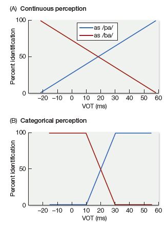
Figure 7.4 Idealized graphs representing two distinct hypothetical results from a phoneme forced-choice identification task. (A) Hypothetical data for a perfectly continuous type of perception, in which judgments about the identity of a syllable gradually slide from /ba/ to /pa/ as VOT values increase incrementally. (B) Hypothetical data for a sharply categorical type of perception, in which judgments about the syllable’s identity remain absolute until the phoneme boundary, where the abruptly shift. Many consonants that represent distinct phonemes yield results that look more like (B) than (A); however, there is variability depending on the specific task and specific sounds.

A slew of studies dating back to 1957 (in work by Mark Liberman and his colleagues) seems to support the claim of categorical perception. One common way to test for categorical perception is to use a forced-choice identification task. The strategy is to have people listen to many examples of speech sounds and indicate which one of two categories each sound represents (for example, /pa/ versus /ba/). The speech sounds are created in a way that varies the VOT in small increments—for example, participants might hear examples of each of the two sounds at 10-ms increments, all the way from –20 ms to 60 ms. (A negative VOT value means that vocal fold vibration begins even before the release of the articulators.)

If people were paying attention to each incremental adjustment in VOT, you’d find that at the extreme ends (i.e., at –20 ms and at 60 ms), there would be tremendous agreement about whether a sound represents a /ba/ or a /pa/, as seen in Figure 7.4A. In this hypothetical figure, just about everyone agrees that the sound with the VOT at –20 ms is a /ba/, and the sound with the VOT at 60 ms is a /pa/. But, as also shown in Figure 7.4A, for each step away from –20 ms and closer to 60 ms, you see a few more people calling the sound a /pa/.

But when researchers have looked at people’s responses in forced-choice identification tasks, they’ve found a very different picture, one that looks more like the graph in Figure 7.4B. People agree pretty much unanimously that the sound is /ba/ until they get to the 20-ms VOT boundary, at which point the judgments flip abruptly. There doesn’t seem to be much mental argument going on about whether to call a sound /ba/ or /pa/. (The precise VOT boundary that separates voiced from unvoiced sounds can vary slightly, depending on the place of articulation of the sounds.) In fact, chinchillas show a remarkably similar pattern (see Box 7.3), suggesting that this way of sorting sounds is not dependent on human capacity for speech or experience with it.

But do studies like these truly tap into the perception of speech sounds—or something else, like decisions that people make about speech sounds, which could be quite different from what they’re doing when they’re perceiving speech in real-time conversation? More recently, researchers have questioned the categorical nature of perception. One such study, led by Bob McMurray (2008), showed that people often do experience quite a bit of uncertainty about whether they’ve heard a voiced or a voiceless sound—much as you might have felt uncertain about the sorting of objects into cups and bowls in Figure 7.2— and that the degree of uncertainty depends on details of the experimental task. Figure 7.6 shows the results of two versions of their experiment. One version, Experiment A, involved a classic forced-choice identification task: participants heard nine examples of the syllables /ba/ and /pa/ evenly spaced along the VOT continuum, and pressed buttons labeled “b” or “p” to show which sound they thought they’d heard. The results (which reflect the percentage of trials on which they pressed the “p” button) show a typical categorical perception curve, with a very steep slope right around the VOT boundary. But the results look very different for Experiment B. In this version, the slope around the VOT boundary is much more graded, looking much more like the graph depicting continuous perception in Figure 7.4A, except at the very far ends of the VOT continuum. This task differed from Experiment A in an important way. Rather than categorizing the meaningless syllables “ba” or “pa,” participants heard actual words, such as “beach” or “peach,” while looking at a computer screen that showed images of both possibilities, and then had to click on the image of the word they thought they’d heard. Like the syllables in Experiment A, these words were manipulated so that the voiced/voiceless sounds at their beginnings had VOTs that were evenly spaced along the VOT continuum.

images BOX 7.3

Categorical perception in chinchillas

How much of speech perception is specifically about speech? Does our tendency to sharply categorize speech sounds stem from our capacity for speech, or is this about how our auditory system deals with sound more generally? One way to answer this question is to see how animals process speech sounds. But how can you study speech perception in animals? As with babies, scientists have had to find a way to leverage behaviors that come naturally to animals and incorporate these behaviors into their experiments. Speech scientists Patricia Kuhl and James Miller (1975) took advantage of the fact that in many lab experiments, animals have shown that they can readily link different stimuli with different events, and that they can also learn to produce different responses to different stimuli in order to earn a reward.

In Kuhl and Miller’s study, chinchillas (see Figure 7.5A) heard various speech sounds as they licked a drinking tube to get dribbles of water. When the syllable /da/ was played (with a VOT of 0 ms), it was soon followed by a mild electric shock. As would you or I, the chinchillas quickly learned to run to the other side of the cage when they heard this sound. On the other hand, when the syllable /ta/ came on (with a VOT of 80 ms), there was no electric shock, and if the chinchillas stayed put and continued to drink, they were rewarded by having the water valve open to allow a stronger flow of water. In this way, the researchers encouraged the chinchillas to link two very different events to the different phonemic categories, a distinction the chinchillas were able to make.

The next step was to systematically tweak the voice onset times of the speech stimuli to see how well the chinchillas were able to detect differences between the two sounds at different points along the VOT continuum. Even though the animals had only heard examples of sounds at the far ends of the VOT spectrum, they showed the same tendency as human adults and babies do—that is, to sort sounds into clear-cut boundaries—and the sharp boundary between categories occurred at almost the same VOT as was found for humans (33.5 ms versus 35.2 ms; see Figure 7.5B). In fact, many languages make a phonemic distinction between sounds that roughly span this boundary. This suggests that some of the phonemic contrasts found in languages may be rooted in the basic nature of auditory stimuli and the general hearing apparatus that we share with our mammalian relatives.

Figure 7.5 (A) Chinchillas are rodents about the size of a squirrel. They are a good choice for auditory studies because their range of hearing (20–30 kHz) is close to that of humans. (B) Results from Kuhl and Miller’s categorical perception experiment, comparing results from the animals and human adults. The graph shows the mean percentage of trials in which the stimulus was treated as an instance of the syllable /da/. For humans, this involved asking the subjects whether they’d heard a /da/ or /ta/ sound; for chinchillas, it involved seeing whether the animals fled to the other side of the cage or stayed to drink water. (A photo by David McIntyre; B after Kuhl & Miller, 1975, Science 190, 69.)

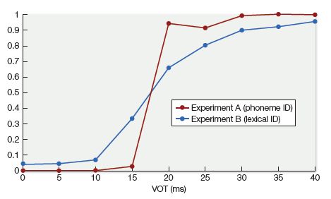
Figure 7.6 Proportion of trials identified as /p/ as a function of VOT for Experiment A, which involved a forced-choice identification task where subjects had to indicate whether they heard /ba/ or /pa/, and Experiment B, a word recognition task in which subjects had to click on the image that corresponded to the word they heard (e.g., beach or peach). (After McMurray et al., 2008, J. Exp. Psych.: Hum. Percep. Perform. 34, 1609.)

McMurray and his colleagues argued that matching real words with their referents is a more realistic test of actual speech perception than making a decision about the identity of meaningless syllables—and therefore that true perception is fairly continuous, rather than warped to minimize differences within categories. But does this mean that we should dismiss the results of syllable-identification tasks as the products of fatally flawed experiments, with nothing to say about how the mind interprets speech sounds? Not necessarily. The syllable-identification task may indeed be tapping into something psychologically important that’s happening at an abstract level of mental representation, with real consequences for language function (for example, for making generalizations about how sounds pattern in your native tongue) but without necessarily warping perception itself.

This is one of those occasions when brain-imaging experiments can be helpful in untangling the debate. As you saw in Chapter 3, language function is distributed across many different regions of the brain and organized into a number of networks that perform a variety of language-related tasks. The duties of one brain network might rely on preserving acoustic details, whereas those of another might privilege the distinctions between abstract categories while downplaying graded differences within categories.

An fMRI study led by Emily Myers (2009) suggests that this line of thinking is on the right track. The design of the study leveraged a phenomenon known as repetition suppression, which is essentially the neural equivalent of boredom caused by repetition. When the same sound (e.g., “ta”) is played over and over again, brain activity in the neural regions responsible for processing speech sounds start to drop off; activity then picks up again if a different sound (e.g., “da”) is played. But what happens if a repeated “ta” sound is followed by another “ta” sound that has a different VOT value than the first, but is still a member of the same phonemic category? Will there be a re-firing up of neural activity just as with the clearly different sound “da”? If the answer is yes, this suggests that the brain region in question is sensitive to detailed within-category differences in speech sounds. If the answer is no, it suggests that this particular brain region is suppressing within-category differences and is sensitive mainly to differences across phonemic boundaries.

According to Myers and her colleagues, the answer is: both. Some areas of the brain showed an increase in activation upon hearing a different variant of the same category (compared with hearing yet another identical example of the original stimulus). In other words, these regions were sensitive to changes in VOT even when the two sounds fell within the same phonemic category. But other regions were mainly sensitive to VOT differences across phonemic boundaries, and less so to differences within categories. The locations of these regions provide a hint about how speech processing is organized. Sensitivity to detailed VOT within-category differences was mostly evident within the left superior temporal gyrus (STG), an area that is involved in the acoustic processing of speech sounds. In contrast, insensitivity to within-category differences was evident in the left inferior frontal sulcus, an area that is linked to coordinating information from multiple information sources and executing actions that meet specific goals. This suggests that, even though our perception is finely tuned to detailed differences in speech sounds, we can also hold in our minds more categorical representations and manipulate them to achieve certain language-related goals. Much of speech perception, then, seems to involve toggling back and forth between these different representations of speech sounds, constantly fine-tuning the relationship between them. This helps to explain why the evidence for categorical perception has been so variable, as discussed further in Method 7.1.

images METHOD 7.1 images

What can we learn from conflicting results?

Many people find it deeply frustrating to read about a study whose results contradict those of an earlier experiment. For some, the conflict raises doubts about scientists’ competence or even the possibility that science can ever truly find reliable answers. Others may just decide they’d rather not cope with the uncertainty and confusion and proceed to tune out the scientific discussion. This is unfortunate because conflicting results don’t always mean that the phenomenon of interest isn’t real (or knowable), but often point to new questions that should be asked and explored for a fuller understanding of a very real phenomenon. In medical research, for example, initial failures to replicate earlier studies have sometimes led to the discovery of important differences in the effects of medications on women versus men.

Over the long history of research in categorical perception, many studies have shown evidence for sharp boundaries for certain sound distinctions, whereas others have shown more continuous patterns of perception. The least intelligent response to this is to count the number of published experiments on either side to see which result is “right.” The point of scientific progress, after all, is to come to a conclusion that is less wrong than previous ones. Inconsistent results can provide critical clues about the specific conditions under which a phenomenon such as categorical perception can be observed, and this gives us important information about its nature.

In psycholinguistics, it’s extremely common to find dramatically different results as a result of what seem like slight differences in a task. For example, a number of researchers have found different results between the forced-choice identification task and the ABX discrimination task, in which two different sounds (e.g., /pa/ and /ba/) are played, followed by a third (either /pa/ or /ba/). The hearer has to decide whether the third sound is the same as the first or the second. And, as you’ve seen, Bob McMurray and his colleagues found evidence of fairly continuous perception when they were asked to identify which of two similar words (e.g., peach or beach) they’d heard.

At first glance, all of these tasks can be reasonably lumped into the category of “speech perception”: in all cases, the hearer has to map an acoustic property onto some linguistically relevant sound category. But think a bit more about whether other cognitive processes are at work in these tasks. The forced-choice identification task requires hearers to compare the target (e.g., /pa/) with their representation in long-term memory of what /pa/ and /ba/ sound like and decide whether the target is more similar to one or the other. The ABX discrimination task forces the hearer to rely on short-term memory to keep track of which sounds were produced in which sequence.

Both of these tasks require subjects to consciously direct their attention to the speech sounds they’re hearing, and in this sense, they may both differ from the word choice task set up by McMurray and colleagues—here, the hearer’s task might be described as mapping the incoming sounds onto a word representation (a process you’ll learn more about in the following chapter) and then indicating the degree of confidence in one choice or another. This could arguably be done without the hearer consciously attending to the first sound in the word and deciding whether it’s a /p/ or a /b/ sound. Decomposing these experimental tasks more accurately into the entire set of cognitive jobs that each task requires might make it less mysterious why categorical perception effects emerge more strongly in some situations than in others. All of these tasks require speech perception—plus something else. Does speech perception itself strip away linguistically irrelevant phonetic detail, or is the process part of the “something else”? It’s only by taking a serious look at seemingly contradictory results that we’ll be able to answer this question. It may well turn out that categorical perception is not needed for understanding speech in normal situations (and, as you’ll see in later sections and chapters, maintaining detailed representations of sounds could be advantageous); but it may well prove to be critical for other speech-related tasks—possibly even for learning to read, as explored in the Digging Deeper section of this chapter.

7.2 Integrating Multiple Cues

In the previous section, I may have given you the impression that the difference between voiced and voiceless sounds can be captured by a single acoustic cue, that of VOT. But that’s a big oversimplification. Most of the studies of categorical perception have focused on VOT because it’s easy to manipulate in the lab, but out in the real, noisy, messy world, the problem of categorizing sounds is far more complex and multidimensional. According to Leigh Lisker (1986), the distinction between the words rapid and rabid, which differ only in the voicing of the middle consonant, may be signaled by about sixteen different acoustic cues (and possibly more). In addition to VOT, these include: the duration of the vowel that precedes the consonant (e.g., the vowel in the first syllable is slightly longer for rabid than rapid); how long the lips stay closed during the “p” or “b” sound; the pitch contour before and after the lip closure; and a number of other acoustic dimensions that we won’t have time to delve into in this book. None of these cues is absolutely reliable on its own. On any given occasion, they won’t all point in the same direction—some cues may suggest a voiced consonant, whereas others might signal a voiceless one. The problem for the listener, then, is how to prioritize and integrate the various cues.

A multitude of acoustic cues

Listeners don’t appear to treat all potentially useful cues equally; instead, they go through a process of cue weighting, learning to pay attention to some cues more than others (e.g., Holt & Lotto, 2006). This is no simple process. It’s complicated by the fact that some cues can serve a number of different functions. For example, pitch can help listeners to distinguish between certain phonemes, but also to identify the age and sex of the talker, to read the emotional state of the talker, to get a sense of the intent behind an utterance, and more. And sometimes, it’s just noise in the signal. This means that listeners might need to adjust their focus on certain cues depending on what their goals are. Moreover, the connection between acoustic cues and phonemic categories will vary from one language to another, and within any given language, from one dialect to another, and even from one talker to another—and even within a single talker, on how quickly or informally that person is speaking.

We don’t yet have a complete picture of how listeners weight perceptual cues across the many different contexts in which they hear speech, but a number of factors likely play a role. First, some cues are inherently more informative than others and signal a category difference more reliably than other cues. This itself might depend upon the language spoken by the talker—VOT is a more reliable cue to voicing for English talkers then it is for Korean talkers, who also rely heavily on other cues, such as pitch at vowel onset and the length of closure of the lips (Schertz et al., 2015). It’s obviously to a listener’s advantage to put more weight on the reliable cues. Second, the variability of a cue matters: if the acoustic difference that signals one category over another is very small, it might not be worth paying much attention to that cue. On the other hand, if the cue is too variable, with wildly diverging values between members of the same category, then listeners may learn to disregard it. Third, the auditory system may impose certain constraints, so that some cues are simply easier to hear than others. Finally, some cues are more likely to be degraded than others when there’s background noise, so they may be less useful in certain environments, or they may not be present in fast or casual speech.

The problem of cue integration has prompted a number of researchers to build sophisticated models to try to simulate how humans navigate this complex perceptual space (for example, see Kleinschmidt, 2018; Toscano & McMurray, 2010). Aside from figuring out the impact of the factors I’ve just mentioned, these researchers are also grappling with questions such as: How much experience is needed to settle on the optimal cue weighting? How flexible should the assignment of cue weights be in order to mirror the extent to which humans can (or fail to) reconfigure cue weights when faced with a new talker or someone who has an accent? How do higher-level predictions about which words are likely to be uttered interact with lower-level acoustic cues? To what extent do listeners adapt cue weights to take into account a talker’s speech rate?

These models have traveled a long way from the simpler picture presented at the beginning of this chapter—specifically, the idea that stable speech perception is achieved by warping perceptual space to align with category boundaries along a single, critical acoustic dimension. The idea of categorical perception was based on the ideas that it could be useful to ignore certain sound differences; but when we step out of the speech lab and into the noisy and changeable world in which we perceive speech on a daily basis, it becomes clear how advantageous it is to have a perceptual system that does exactly the opposite—one that takes into account many detailed sound differences along many different dimensions, provided it can organize all this information in a way that privileges the most useful information. Given the complexity of the whole enterprise, it would not be surprising to find that there are some notable differences in how individual listeners have mentally organized speech-related categories. Section 7.3 addresses how different experiences with speech might result in different perceptual organization, and Box 7.4 explores the possible impact of experience with music.

images BOX 7.4

Does music training enhance speech perception?

There may be some significant overlap between brain functions for music and language, as explored in the Digging Deeper section of Chapter 3. If that’s the case, could musical practice fine-tune certain skills that are useful for language? Speech perception is a great area in which to explore this question, given that musicians need to be sensitive to a variety of rhythmic and pitch-based cues, and they have to be able to zoom in on some cues and disregard others.

A number of studies comparing musicians to non-musicians do suggest that musicians have heightened abilities when it comes to speech perception. Musicians have been found to have an advantage in accurately perceiving speech embedded in noise (e.g. Parbery-Clark et al., 2009; Swaminathan et al., 2015)—with percussionists showing a stronger advantage than vocalists (Slater & Kraus, 2016). Musical training has also been connected with an improved ability to detect differences between sounds from a foreign language (Martínez-Montes et al., 2013) and with the detection of syllable structure and rhythmic properties of speech (Marie et al., 2011).

These results are intriguing, but on their own, they don’t justify the conclusion that musical practice causes improvements in speech perception—it’s entirely possible that people choose to take up music precisely because they have good auditory abilities to start with, abilities that may help them in both musical and linguistic domains. Researchers are on stronger footing if they can show that people’s perception of speech is better after they’ve spent some in musical training than before they started, as found by a study in which high-schoolers who chose a music program as an option developed faster neural responses to speech after two years in their programs—in contrast with students enrolled in a fitness program, who showed no improvement (Tierney et al., 2013). But this still doesn’t completely control for aptitude or interest, and we don’t know whether putting athletes into music lessons they would otherwise avoid would result in the same effects.

The most scientifically rigorous method (though often least practical) is to randomly assign subjects to music training or a control group. A few such studies are beginning to emerge. Jessica Slater and her colleagues (2015) studied two groups of elementary school children who were on a waiting list for a music program. Half of them were randomly assigned to the program, while the other half were given a spot the following year. After 2 years (but not after just 1 year), the first group performed better in a speech-in-noise test than they had before they started the program, and they also performed better than the second group, who at that point had participated on the program for just 1 year.

Similar logic was applied by Christina Zhao and Pat Kuhl (2016), who chose to study the effects of music training on 9-month-olds because babies of this age show a remarkable capacity for perceptual tuning. Half of the babies were randomly assigned to a 4-week, 12-session music program in which they were exposed to waltz-based musical rhythms (chosen because the ONE-two-three rhythm of the waltz is more difficult than rhythms that involve two or four equal beats) while their caregivers played clapping and tapping games with them. The other group was assigned to a program that focused on general motor skills through block-stacking and similar games. At the end of the 4 weeks, the researchers measured the infants’ brain activity using MEG techniques (which are very similar to the EEG methods you read about in Chapter 3). Babies heard sequences of speech sounds that contrasted the syllable ibi with ibbi—a subtle difference in consonant length that is phonemic in some languages, but not in English. The stimuli were structured so that ibi occurred 85 percent of the time, and ibbi only 15% of the time. This structure normally elicits a mismatch response—that is, a spike in brain activity whenever the less frequent (and therefore less expected) sound is encountered. The babies who had been randomly assigned to the music program showed stronger mismatch responses than the control group (see Figure 7.7).

Results like these further bolster the idea that musical skills are intertwined with speech perception. This may be welcome news for people who push back against the current trend of cutting educational costs by eliminating musical programs from school curricula. But advocates for music programs shouldn’t get too carried away with waving these results around to promote their cause. Although suggestive, the studies described here don’t tell us much about how meaningful the effects of musical training might be over the course of people’s lives. Do enhanced brain responses translate into practical advantages in processing linguistic information? And are these effects fairly permanent, or do they quickly evaporate if a child decides to drop music lessons and take up tae kwon do instead? Possibly, the best argument for music education is still that it allows students to participate in making music.

Figure 7.7 Plots of brain wave activity in the temporal (top panel) and prefrontal (bottom panel) regions for the music training and control groups. Values on the y-axis reflect the difference between average wave amplitudes for bibi when it occurred as the unexpected syllable (15 percent of the time) and average wave amplitude for bibi when it occurred as the most frequent, expected syllable (85 percent of the time). (After Zhao & Kuhl, 2016, PNAS 113, 5212.)

Context effects in speech perception

Another way to achieve stable sound representations in the face of variable acoustic cues might be to use contextual cues to infer sound categories. In doing this, you work backward, applying your knowledge of how sounds “shape-shift” in the presence of their neighbors to figure out which sounds you’re actually hearing. It turns out that a similar story is needed to account for perceptual problems other than speech. For example, you can recognize bananas as being yellow under dramatically different lighting conditions, even though more orange or green might actually reach your eyes depending on whether you’re seeing the fruit outdoors on a misty day or inside by candlelight (see Figure 7.8). Based on your previous experiences with color under different lighting conditions, you perceive bananas as having a constant color rather than changing, chameleon-like, in response to the variable lighting. Without your ability to do this, color would be pretty useless as a cue in navigating your physical environment. In the same way, knowing about how neighboring sounds influence each other might impact your perception of what you’re hearing. The sound that you end up “hearing” is the end result of combining information from the acoustic signal with information about the sound’s surrounding context.

An even more powerful way in which context might help you to identify individual sounds is knowing which word those sounds are part of. Since your knowledge of words includes knowledge of their sounds, having a sense of which word someone is trying to say should help you to infer the specific sounds you’re hearing. William Ganong (1980) first demonstrated this phenomenon, lending his name to what is now commonly known as the Ganong effect. In his experiment, subjects listened to a list of words and non-words and wrote down whether they’d heard a /d/ or a /t/ sound at the beginning of each item. The experimental items of interest contained examples of sounds that were acoustically ambiguous, between a /d/ and /t/ sound, and that appeared in word frames set up so that a sound formed a word under either the /d/ or /t/ interpretation, but not both. So, for example, the subjects might hear an ambiguous /d-t/ sound at the beginning of __ask, which makes a real word if the sound is heard as a /t/ but not as a /d/; conversely, the same /d-t/sound would then also appear in a frame like __ash, which makes a real word with /d/ but not with /t/. What Ganong found was that people interpreted the ambiguous sound with a clear bias in favor of the real word, even though they knew the list contained many instances of non-words. That is, they reported hearing the same sound as a /d/ in __ash, but a /t/ in __ask.

Figure 7.8 Color constancy under different lighting. We subjectively perceive the color of these bananas to be the same under different lighting conditions, discounting the effects of illumination. Similar mechanisms are needed to achieve a stable perception of variable speech sounds. (Photographs by David McIntyre.)

This experiment helps to explain why we’re rarely bothered by the sloppiness of pronunciation when listening to real, meaningful speech—we do a lot of perceptual “cleaning up” based on our understanding of the words being uttered. But the Ganong study also revealed limits to the influence of word-level expectations: The word frame only had an effect on sounds that straddled the category boundary between a /t/ and /d/. If the sounds were good, clear examples of one acoustic category or the other, subjects correctly perceived the sound on the basis of its acoustic properties, and did not report mishearing dask as task. This shows that context cues are balanced against the acoustic signal, so that when the acoustic cues are very strong, expectations from the word level aren’t strong enough to cause us to “hallucinate” a different sound. However, when the acoustic evidence is murky, word-level expectations can lead to pretty flagrant auditory illusions). One such illusion is known as the phoneme restoration effect, first discovered by Richard Warren (1970). In these cases, a speech sound is spliced out—for example, the /s/ in legislature is removed—and a non-speech sound, such as a cough, is pasted in its place. The resulting illusion causes people to “hear” the /s/ sound as if it had never been taken out, along with the coughing sound.

Integrating cues from other perceptual domains

You may have noticed, when trying to talk to someone at a loud party, that it’s much easier to have a conversation if you’re standing face to face and can see each other’s face, lips, and tongue. This suggests that, even without special training in lip reading, your knowledge of how sounds are produced in the mouth can help you interpret the acoustic input.

There is, in fact, very clear evidence that visual information about a sound’s articulation melds together with acoustic cues to affect the interpretation of speech. This integration becomes most obvious when the two sources of information clash, pushing the system to an interesting auditory illusion known as the McGurk effect. When people see a video of a person uttering the syllable ga, but the video is accompanied by an audio recording of the syllable ba, there’s a tendency to split the difference and perceive it as the syllable da—a sound that is produced somewhere between ba, which occurs at the front of the mouth, and ga, which is pronounced at the back, toward the throat. This finding is a nice, sturdy experimental effect. It can be seen even when subjects know about and anticipate the effect, it occurs with either words or non-words (Dekle et al., 1992)—and it even occurs when blindfolded subjects feel a person’s lips moving to say ba while hearing recordings of the syllable ga (Fowler & Dekle, 1991).

The McGurk effect offers yet more strong evidence that there is more to our interpretation of speech sounds than merely processing the acoustic signal. What we ultimately “hear” is the culmination of many different sources of information and the computations we’ve performed over them. In fact, the abstract thing that we “hear” may actually be quite separate from the sensory inputs that feed into it, as suggested by an intriguing study by Uri Hasson and colleagues (2007). Their study relied on the repetition suppression phenomenon you read about in Section 7.1, in which neural activity in relevant brain regions becomes muted after multiple repetitions of the same stimuli. (In that section, you read about a study by Emily Myers and her colleagues, who found that certain neural regions responded to abstract rather than acoustic representations of sounds, treating variants of the same phonemic category as the “same” even though they were acoustically different.) Hasson and colleagues used repetition suppression to examine whether some brain regions equate a “ta” percept that is based on a McGurk illusion—that is, based on a mismatch between an auditory “pa” and a visual “ka”—with a “ta” percept that results from accurately perceiving an auditory “ta” with visual cues aligned, that is, showing the articulation of “ta.” In other words, are some areas of the brain so convinced by the McGurk illusion that they ignore the auditory and visual sensory information that jointly lead to it?

They found such an effect in two brain regions, the left inferior frontal gyrus (IFG) and the left planum polare (PP). (Note that the left IFG is also the area in which Myers and her colleagues found evidence for abstract sound representations; the left PP is known to be involved in auditory processing.) In contrast, a distinct area—the transverse temporal gyrus (TTG), which processes detailed acoustic cues—showed repetition suppression only when the exact auditory input was repeated, regardless of whether the perceived sound was the same or not. That is, in the TTG, repetition suppression was found when auditory “pa” combined with visual “pa” were followed by auditory “pa” combined with visual “ka,” even though the second instance was perceived by the participants as “ta” and not “pa.”

7.3 Adapting to a Variety of Talkers

As you’ve seen throughout this chapter, sound categories aren’t neatly carved at the joints. They can’t be unambiguously located at specific points along a single acoustic dimension. Instead, they emerge out of an assortment of imperfect, partly overlapping, sometimes contradictory acoustic cues melded together with knowledge from various other sources. It’s a miracle we can get our smartphones to understand us in the best of circumstances.

The picture we’ve painted is still too simple, though. There’s a whole other layer of complexity we need to add: systematic variation across speakers. What makes this source of variation so interesting is that it is in fact systematic. Differences across talkers don’t just add random noise to the acoustic signal. Instead, the variation is conditioned by certain variables; sometimes it’s the unique voice and speaking style of a specific person, but other predictable sources of variation include the age and gender of the talker (which reflect physical differences in the talker’s vocal tract), the talker’s native language, the city or area they live in, or even (to some extent) their political orientation (see Box 7.5). As listeners, we can identify these sources of variation: we can recognize the voices of individual people, guess their mother tongue or the place they grew up, and infer their age and gender. But can we also use this information to solve the problem of speech perception? That is, can we use our knowledge about the talker—or about groups of similar talkers—to more confidently map certain acoustic cues onto sound categories?

images LANGUAGE AT LARGE 7.1

To dub or not to dub?

Travel to a non-English-speaking country can result in some unsettling cultural experiences, even if you spend much of your time watching TV in your hotel room. It may not have occurred to you to wonder what Captain Kirk would sound like in Slovakian, but—there it is. Such late-night viewing of dubbed programs often arouses my scientific curiosity: How do Slovakian viewers cope with the fact that when they hear Captain Kirk saying the Slovakian version of “Beam me up, Scotty,” his English-moving mouth appears to be saying something that (to them) means “I’d drink some coffee.” Do they listen to Star Trek episodes at a higher volume than their American counterparts to compensate for the fact that they can’t trust the information in the visual channel? Do they learn to re-weight their cues when watching TV to suppress the misleading visual information? If you were to administer a test as the credits were rolling, would you find a temporarily diminished McGurk effect among the viewers of dubbed programs?

While the citizens of many countries are forced to listen to bad dubbing of foreign shows (or read subtitles), Germany takes its dubbing very seriously. According to the Goethe Institute, dubbing became a major enterprise in Germany after World War II, when almost all films screened in German cinemas were foreign (mainly American, French, or British) at a time when the population had negative reactions to hearing these languages, given that they represented the native tongues of their recent foes. To make these films more palatable, they were dubbed into German, giving rise to a highly developed industry that is currently the source of national pride. The ultimate goal for dubbing directors and actors is to produce a version of a film or program that does not appear to be dubbed. Doing so is incredibly difficult. As evident from psycholinguistic experiments, we naturally integrate visual information about how a sound is articulated with the incoming acoustic information, which is why watching most dubbed programs feels so, well, unnatural. This imposes a stringent condition on dubbing that translators of print never have to worry about: how to match up not just the subtle meaning of a translation with its original, but also the articulatory properties of the sounds involved. Very often, the two will clash, leading to difficult choices. For example, suppose an English-speaking character has just uttered the word “you” in a line of dialogue. The German scriptwriter has two possible translation options: the informal du, which is pronounced in a very similar way to “you,” and the formal Sie, in which the vowel requires spreading the lips, rather than rounding them, a visually obvious clash. But what if the character is speaking to a high-status person he’s just met? A German speaker would never say “du” in this situation.

While it’s very hard to achieve dubbing perfection to the point that the dubbing goes unnoticed, it’s possible, with some effort, to achieve impressive results. This is because, while visual information about pronunciation clearly plays a role in the understanding of speech, its role is quite incomplete. Subtle tongue gestures are often only partially visible from behind teeth and lips or—for example, try visually distinguishing the syllables sa, ta, da, and na. And a number of important sound contrasts are not at all visible on the face—such as voicing contrasts, which depend on the vibration of the vocal folds tucked away from view. This gives dubbing artists a fair bit of room in which to maneuver. While this is welcome news for the dubbing industry, it also makes it apparent why “lip-reading” as practiced by people who are deaf is more like “lip-guessing.” The information that is visually available is far less detailed and constraining than the auditory information, forcing the lip-reader to rely heavily on the context, their knowledge base, and lots of fast guessing to fill in the gaps. It’s an uncertain and exhausting process, typically conducted in a non-native language. If you’re a hearing person, this might be a useful analogy: take some ASL courses, then try understanding what someone is signing based on a video in which the hands are blurred out much of the time.

The challenges of lip-reading apparently provided the inspiration for the humorous “Bad Lip Reading” series of videos on YouTube. In an interview with Rolling Stone magazine, the anonymous creator of these videos revealed that his fascination with the topic began when he observed his mother learning to lip-read after losing her hearing in her 40s. The videos cleverly exploit the ample gap between visual and auditory information. By taking footage of TV shows, sports events, or political news and dubbing absurd words over the lip movements of the speakers or singers, the creator treats his public to comedic gems—such as Presidents Trump and Obama exchanging insults during the Trump inauguration of 2018, or a deeply odd episode of the hit series Stranger Things in which Mike and Nancy’s prim mother announces perkily over dinner, “I have a lovely tattoo.”

images BOX 7.5

Accents and attitudes

Have you ever made a snap judgment about someone’s political views based on their clothing (tailored suit, or t-shirt and cargo pants) or their drink order (whatever’s on tap, or 12-year-old Scotch)? It’s no secret among ethnographers that people often tailor their appearance and consumption habits in a way that signals their identification with a certain social group or ideology. The same seems to be true of accents.

The connection between social identity and accent was first noticed by linguist Bill Labov (1972). While visiting the island of Martha’s Vineyard in Massachusetts, Labov noticed that many of the islanders had a unique way of saying words like “rice” and “sight”—they pronounced them higher in the mouth, not quite “roice” and “soight,” but somewhat in that direction. But locals varied quite a bit in terms of how they pronounced their vowels, so Labov set about making painstaking recordings of people from all over the island. He found that the raised “ay” sound was more concentrated in some groups than in others and identified a profile of the typical “ay” raiser. Raising was especially prevalent in the fishing community of Chilmark, especially among fishermen, many of whom were keen on preserving a fading way of life. They looked askance at the “summer people” and newcomers who traipsed around the island as if they owned it. When Labov asked people directly about how proud they felt of their local heritage, and how resentful they were of summer visitors like himself, he found that people who most valued the traditional island lifestyle were the ones who raised their vowels the most. High schoolers who planned to come back to the island after going to college raised their vowels more than those who thought they would build a life away from the island. Most residents of Martha’s Vineyard were not consciously aware that they produced different vowels than the mainlanders, even though they had a general sense that their accent was different from the mainland accent. They subconsciously used their vowels as a subtle badge of identity.

More recently, Labov (2010) has tracked a linguistic change that’s occurring in the northern region of the U.S. clustering around the Great Lakes. This dialect region, called the Inland North, runs from just west of Albany to Milwaukee, loops down to St. Louis, and traces a line to the south of Chicago, Toledo, and Cleveland. Thirty-four million speakers in this region are in the midst of a modern-day rearrangement of their vowel system. Labov thinks it started in the early 1800s, when the linguistic ancestors of this new dialect began to use a distinct pronunciation for the vowel in “man,” such that it leaned toward “mee-an.” This eventually triggered a free-for-all game of musical chairs involving vowels. The empty slot left by this first vowel shift was eventually filled by the “o” sound, so that “pod” came to be pronounced like “pad” used to be; then “desk” ended up being pronounced like the former “dusk,” “head” like “had,” “bus” like “boss,” and “bit” like erstwhile “bet.”

Genuine misunderstandings arise when speakers of this dialect encounter listeners who are not familiar with it. Labov describes the following situation, reconstructed from an incident reported in the Philadelphia Inquirer:

Gas station manager: It looks like a bomb on my bathroom floor.

Dispatcher: I’m going to get somebody. (That somebody included the fire department.)

Manager: The fire department?

Dispatcher: Well yes, that’s standard procedure on a bomb call.

Manager: Oh no, ma’am, I wouldn’t be anywhere near a bomb. I said I have a bum on the bathroom floor.

Eight firefighters, three sheriff’s deputies, and the York County emergency preparedness director showed up at the gas station to escort the homeless transient out.

One of the puzzles about this vowel shift is why it has spread through an area of 88,000 square miles only to stop cold south of Cleveland and west of Milwaukee. Labov points out that the residents of the Inland North have long-standing differences with their neighbors to the south, who speak what’s known as the Midland dialect. The two groups originated from distinct groups of settlers; the Inland Northerners migrated west from New England, whereas the Midlanders originated in Pennsylvania via the Appalachian region. Historically, the two settlement streams typically found themselves with sharply diverging political views and voting habits, with the Northerners generally being more liberal. Labov suggests that it’s these deep-seated political disagreements that create an invisible borderline barring the encroachment of Northern Cities Vowels. When he looked at the relationship between voting patterns by county over the three previous presidential elections and the degree to which speakers in these counties shifted their vowels, he found a tight correlation between the two.

Do vowel-shifters sound more liberal to modern ears? Yes, at least to some extent. Labov had students in Bloomington, Indiana, listen to a vowel-shifting speaker from Detroit and a non-vowel-shifter from Indianapolis. The students rated the two speakers as equal in probable intelligence, education, and trustworthiness. But they did think the vowel-shifting speaker was more likely to be in favor of gun control and affirmative action.

Are we moving toward an era where Americans will speak discernibly “red” or “blue” accents? It’s hard to say, but linguists like Bill Labov have shown that American dialects have been pulling apart from each other, with different dialectal regions diverging over time rather than converging—yet one more polarizing development that is making conversations between fellow Americans increasingly challenging.

Evidence for adaptation

Variation across talkers is significant enough to pose a real challenge for speech perception. For example, Figure 7.9 shows the distribution of /s/ and /ʃ/ (as in the words sip versus ship) along one of the important acoustic cues that distinguish these two sounds. As you can see, these distributions are quite different from each other, with one talker’s /ʃ/ sounds overlapping heavily with the other person’s /s/ sounds. How do listeners cope with such variation? Do they base their sound categories on the average distributions of all the talkers they’ve ever heard? If so, talkers who are outliers might be very hard to understand. Or do listeners learn the various speech quirks of individual talkers and somehow adjust for them?

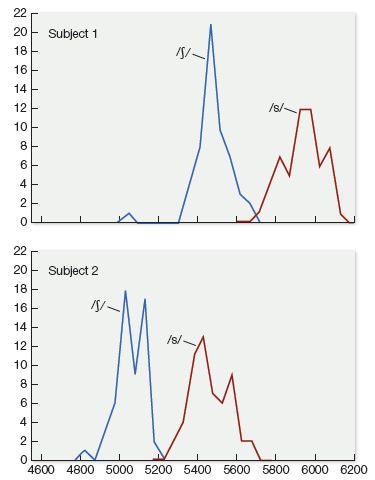
Figure 7.9 Distribution of frication frequency centroids, an important cue for distinguishing between /s/ and /ʃ/, from two different talkers; note the considerable overlap between the sound /ʃ/ for subject ACY and the sound /s/ for subject IAF. (From Newman et al., 2001, J. Acoust. Soc. Am. 109, 1181.)

People do seem to tune their perception to individual talkers. This was observed by speech scientists Lynne Nygaard and David Pisoni (1998), who trained listeners on sentences spoken by 10 different talkers over a period of 3 days, encouraging listeners to learn to label the individual voices by their assigned names. At the end of the 3-day period, some listeners heard and transcribed new sentences, recorded by the same ten talkers and mixed with white noise, while other listeners were tested on the same sentences (also mixed with noise) spoken by a completely new set of talkers. Those who transcribed the speech of the familiar talkers performed better than those tested on the new, unfamiliar voices—and the more noise was mixed into the signal, the more listeners benefitted from being familiar with the voices.

These results show that speech perception gets easier as a result of experience with individual voices, especially under challenging listening conditions, suggesting that you’ll have an easier time conversing at a loud party with someone you know than someone you’ve just met. But Nygaard and Pisoni’s results don’t tell us how or why. Does familiarity help simply because it sharpens our expectations of the talker’s general voice characteristics (such as pitch range, intonation patterns, and the like), thereby reducing the overall mental load of processing these cues? Or does it have a much more precise effect, helping us to tune sound categories based on that specific talker’s unique way of pronouncing them?

Researchers at Work 7.1 describes an experiment by Tanya Kraljic and Arthur Samuel (2007) that was designed to test this question more precisely. This study showed that listeners were able to learn to categorize an identical ambiguous sound (halfway between /s/ and /ʃ/) differently, based on their previous experience with a talker’s pronunciation of these categories. What’s more, this type of adaptation is no fleeting thing. Frank Eisner and James McQueen (2008) found that it persisted for at least 12 hours after listeners were trained on a mere 4-minute sample of speech.

The same mechanism of tuning specific sound categories seems to drive adaptation to unfamiliar accents, even though the speech of someone who speaks English with a marked foreign accent may reflect a number of very deep differences in the organization of sound categories, and not just one or two noticeable quirks. In a study by Eva Reinisch and Lori Holt (2004), listeners heard training words in which sounds that were ambiguous between /s/ and /f/ were spliced into the speech of a talker who had a noticeable Dutch accent. (As in other similar experiments, such as the one by Kraljic and Samuel, these ambiguous sounds were either spliced into words that identified the sound as /s/, as in harness, or /f/, as in belief). Listeners adjusted their categories based on the speech sample they’d heard, and, moreover, carried these adjustments over into their perception of speech produced by a different talker who also had a Dutch accent. So, despite the fact that the Dutch speakers differed from the average English speaker on many dimensions, listeners were able to zero in on this systematic difference, and generalize across accented talkers. Note, however, that the systematic production of an ambiguous /s/-/f/ sound as either /s/ or /f/ was an artificial one in this experiment—it doesn’t reflect an actual Dutch accent, but was used for the purpose of this experiment because it allowed the researchers to extend a finding that was well established in studies of adaptation to individual talkers to the broader context of adaptation to foreign accents. Reassuringly, similar effects of listener adaptation have been found for real features of accents produced naturally by speakers—as in, for example, the tendency of people to pronounce voiced sounds at the ends of words as voiceless (pronouncing seed as similar to seat) if they speak English with a Dutch or Mandarin accent (Eisner et al., 2013; Xie et al., 2017).

images RESEARCHERS AT WORK 7.1

Adjusting to specific talkers

Source: Experiment 2 in T. Kraljic & A. G. Samuel. (2007) Perceptual adjustments to multiple speakers. Journal of Memory and Language 56, 1–15.

Question: Do listeners learn to adjust phonemic boundaries in a way that takes into account the pronunciations of individual talkers?

Hypothesis: Participants who are exposed to an ambiguous sound halfway between /s/ and /ʃ/ that functions as /s/ for one talker but /ʃ/ for a second talker will shift their phonemic boundaries accordingly, so that ambiguous sounds are more likely to be categorized as /s/ for the first talker but /ʃ/ for the second.

Test: Forty-eight adults with normal hearing who were native speakers of English participated in a two-phase experiment. In the exposure phase, participants listened to 100 words and 100 non-words. and for each item were asked to decide whether it was a real word or not by pressing one of two buttons. Among the real words, 20 key items contained the /s/ phoneme (e.g., hallucinate) and 20 contained the /ʃ/ phoneme (e.g., negotiate); the other words were distractors. Half of the items, including the key items, were spoken by a male voice and the other half by a female voice, so that each participant heard 10 /s/ words and 10 /ʃ/ words spoken by the male and 10 /s/ words and 10 /ʃ/ words spoken by the female. Participants were randomly assigned to one of two groups. For one group, all the /s/ words spoken by the male contained a clear, typical example of /s/, whereas all the /ʃ/ words contained a spliced-in ambiguous sound halfway between /s/ and /ʃ/. Conversely, the female voice produced all of the /s/ words with the (same) ambiguous sound, but all of the /ʃ/, words with a clear, typical example of /ʃ/. The situation was reversed for the second group of participants, so that the male voice uttered the ambiguous sound only in the /s/ words (with typical /ʃ/ sounds in the /ʃ/ words), whereas the female voice uttered the ambiguous sound only in the /ʃ/ words (with typical /s/ sounds in the /s/ words).

If listeners adapt to individual talkers’ pronunciations rather than just averaging acoustic information out across talkers, then they should carve the sound space up differently for each voice. This was tested during the categorization phase: All participants heard both the male and female voice producing six stimulus items on a continuum from /asi/ to /aʃi/, with the items representing equal steps along this continuum. They had to indicate whether they thought each item contained the sound /s/ (by pressing a button labelled “S”) or the /ʃ/ sound (by pressing a button labelled “SH”). The order of the male and female voices was counterbalanced across subjects.

Results: Performance on the categorization task depended on what participants heard in the exposure phase. Figure 7.10 shows the percentage of categorizations as /ʃ/, with the data collapsed across male and female voices and exposure groups. The graph shows that participants were more likely to categorize an intermediate sound as /ʃ/ for a particular voice if the ambiguous sound had appeared in /ʃ/ words uttered by that same talker. For example, those who had heard the female voice utter the ambiguous sound in /ʃ/ words (but not in /s/ words) during the exposure phase were more likely to say that the intermediate examples of the stimuli were /ʃ/ sounds than those who had heard the female voice utter the ambiguous sound in /s/ words. This occurred despite the fact that the participants heard an equal number of ambiguous sounds uttered as /s/ words by the male voice, a fact that they appeared to disregard when making categorization judgments about the female voice.

Conclusions: Under at least some conditions, adult hearers can shift a phonemic boundary to take into account the speech patterns of individual speakers, even when presented with conflicting speech patterns by a different talker. When native speakers of English heard a specific talker produce a sound that was ambiguous between /s/ and /ʃ/ in words that revealed the sound’s phonemic function, their categorization of sounds along the /s/-/ʃ/ continuum reflected a bias toward the phonemic structure apparent for that talker, even though they heard words from a different talker that showed exactly the opposite bias. This adaptation occurred after only ten examples from that talker of words that clarified the phonemic status of the ambiguous sound.

Questions for further research

1. Would similar adaptation effects be found for other phonemic contrasts? (In fact, a version of this experiment was conducted by Kraljic and Samuel—their Experiment 1, reported in the same article—that did not show talker-specific adaptation for the /t/-/d/ contrast).

2. Would listeners show evidence of adapting to specific talkers if their identity were signaled in some way other than gender—for example, for two male voices of different ages, or two female voices with different accents?

3. Does this adaptation effect depend on having very extensive experience with a language? For example, would it occur if, instead of testing native English listeners, we tested listeners of other languages who had learned English fairly recently?

Figure 7.10 The percentage of “SH” categorizations of stimuli along the /s/-/ʃ/ continuum for words produced by the same voice in the exposure phase. For example, for judgments made about the male voice, the cases labeled as “?SH training” refer to judgments made by participants who heard the male voice produce the ambiguous sound in /ʃ/ words, but not in /s/ words, whereas the “?S training” cases refer to judgments made by participants who heard the male voice produce the ambiguous sound in /s/ words. The data here are collapsed across categorization judgments for both male and female voices. (From Kraljic & Samuel, 2007, J. Mem. Lang. 56, 1.)

Relationships between talker variables and acoustic cues

To recap the story so far, this chapter began by highlighting the fact that we carve a graded, multidimensional sound space into a small number of sound categories. At some level, we treat variable instances of the same category as equivalent, blurring their acoustic details. But some portion of the perceptual system remains sensitive to these acoustic details—without this sensitivity, we probably couldn’t make subtle adjustments to our sound categories based on exposure to individual hearers or groups of hearers whose speech varies systematically.

Researchers now have solid evidence that such adjustments can be made, in some cases very quickly and with lasting effect. But they don’t yet have a full picture of the whole range of possible adjustments. It’s complicated by the fact listeners don’t always respond to talker-specific manipulations in the lab by shifting their categories in a way that mirrors the experimental stimuli. For example, Kraljic and Samuel (2007) found that although listeners adjusted the /s/- /ʃ/ border in a way that reflected the speech of individual talkers, they did not make talker-specific adjustments in response to the VOT boundary between /d/ and /t/. Similarly, Reinisch and Holt (2014) found that listeners extended their new categories from one Dutch-accented female speaker to another female speaker, but did not generalize when the new talker was a male who spoke with a Dutch accent. Why do some adaptations occur more readily than others?

Some researchers argue that the answer to this question lies—at least in part—in the structure that is intrinsic to speech itself. That is, some acoustic cues are very closely tied to the identities of speakers, whereas others are not. Figure 7.11 shows the distribution of two very different cues, one that’s relevant for identifying the vowel /i/ as in beet, and the other (VOT) that’s used to identify voiceless stops like /t/. The distribution averaged across all talkers is contrasted with the distributions for male and female talkers. As you can see, the cue shown in Figure 7.11A shows very different distributions for male versus female speakers; in this case, knowing the gender of the speaker would be very useful for interpreting the cue, and a listener would do well to be cautious about generalizing category structure from a male speaker to a female, or vice versa. In contrast, the VOT cue as depicted in Figure 7.11B does not vary much by gender at all, so it wouldn’t be especially useful for listeners to link this cue with gender. (In fact, for native speakers of English, VOT turns out to depend more on how fast someone is speaking than on who they are.) So, if listeners are optimally sensitive to the structure inherent in speech, they should pay attention to certain aspects of a talker’s identity when interpreting some cues, but disregard talker variables for other cues.

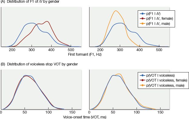
Figure 7.11 (A) Gender-specific distributions (red and yellow lines) of the first vowel formant (F1) for the vowel /i/ are strikingly different from overall average distributions (blue lines). (B) Gender-specific distributions of VOT for voiceless stops diverge very little from the overall distribution. This makes gender informative for interpreting vowel formants, but not for interpreting VOT. (From Kleinschmidt, 2018, PsyArXiv.com/a4ktn/.)

The relationship between talker variables and acoustic cues can be quite complicated; there are several possibly relevant variables and the relationship between a cue and a certain talker variable could be specific to an individual sound. For example, Figure 7.12 shows that it would be extremely useful to know that a speech sample comes from the Northern dialect in the United States if you’re interpreting the vowel formant cues associated with the vowels in cat and Bob—but much less relevant for categorizing the vowels in hit or boot. On the other hand, your interpretation of boot (but not of cat) would be significantly enhanced by knowing that a talker has a New England accent.

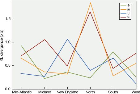
Figure 7.12 Degree of acoustic divergence for each vowel by dialect, based on first and second vowel formants (important cues for vowel identification). This graph shows that dialect distinguishes some vowel formant distributions more than others. In particular, the pronunciation of /æ/ as in cat and /ɑ/ as in father by Northern talkers diverge more than any other vowel/dialect combination. The five most distinct vowel/dialect combinations are shown here. (From Kleinschmidt, 2018, PsyArXiv.com/a4ktn/.)

Complicating matters even further is that, as discussed in Section 7.2, a single sound dimension (such as voicing) is often defined not by a single cue, but by a number of different cues that have to be appropriately weighted. To adapt to new talkers, listeners may have to learn to map a whole new set of cue values to a category—but even more than that, they may have to learn how to re-weight the cues. This was the case for the successful adaptation of English-speaking listeners to Mandarin-accented speech, in a study led by Xin Xie (2017). In this study, listeners had to adjust their sound categories to reflect the fact that the talker produced voiced sounds like /d/ at the ends of words with a VOT that resembled a native English /t/. Aside from VOT, English speakers use other cues to signal voicing at the ends of words. These include the length of the preceding vowel (longer in cad than in cat) and closure duration—that is, the amount of time that the articulators are fully closed (longer in cat than in cad). But the Mandarin-accented talker did not use either of these as a reliable cue for distinguishing between voiced and voiceless sounds. Instead, he relied on burst duration as a distinct cue—that is, the duration of the burst of noise that follows the release of the articulators when a stop is produced (see Figure 7.13). English listeners who heard the Mandarin-accented talker (rather than the same words by the native English speaker) came to rely more heavily on burst duration as a cue when deciding whether a word ended in /d/ or /t/. After just 60 relevant words by this talker, listeners had picked up on the fact that burst duration was an especially informative acoustic cue, and assigned it greater weight accordingly.

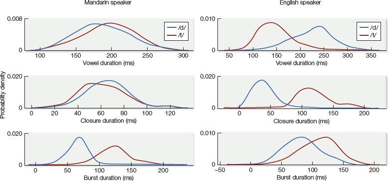
Figure 7.13 Distributions showing the reliance by a Mandarin speaker (left panel) and a native English speaker (right panel) on various acoustic cues (duration of preceding vowel, closure duration and burst duration) when pronouncing 60 English words ending in /d/ or /t/. (From Xie et al., 2017, J. Exp. Psych.: Hum. Percep. Perform. 43, 206.)

The role of a listener’s perceptual history

To begin my Ph.D. studies, I moved to Rochester, New York, from Ottawa, Canada. I became friends with a fellow graduate student who had moved from California. Amused by my Canadian accent, he would snicker when I said certain words like about and shout. This puzzled me, because I didn’t think I sounded any different from him—how could he notice my accent (to the point of amusement) if I couldn’t hear his? After a few months in Rochester, I went back to Ottawa to visit my family, and was shocked to discover that they had all sprouted Canadian accents in my absence. For the first time, I noticed the difference between their vowels and my Californian friend’s.

This story suggests two things about speech perception: first, that different listeners with different perceptual histories can carve up phonetic space very differently from each other, with some differences more apparent to one person than another; and second, that the same listener’s perceptual organization can change over time, in response to changes in their phonetic environment. This makes perfect sense if, as suggested earlier, listeners are constantly learning about the structure that lies beneath the surface of the speech sounds they hear. Because I was exposed (through mass media’s broadcasting of a culturally dominant accent) to Californian vowels much more than my friend was exposed to Canadian ones, I had developed a sound category that easily embraced both, whereas my friend perceived the Canadian vowels as weird outliers. And the distinctiveness of the Canadian vowels became apparent to me once they were no longer a steady part of my auditory diet.

Is there an optimal perceptual environment for learners? You might think that being exposed to highly variable pronunciation would be confusing for language learners—after all, how can you possibly develop a stable representation of a sound if its borders and relevant acoustic cues shift dramatically depending on who’s talking? But being forced to cope with a variety of accents may keep sound representations from settling into categories that are too stable. In a study led by Melissa Baese-Berk (2013), listeners were exposed to sentences produced by five non-native speakers of English, each from a different language background (Thai, Korean, Hindi, Romanian, and Mandarin). After this training session, they listened to and transcribed sentences produced by a new Mandarin-accented talker (i.e., an unfamiliar speaker of a familiar accent) and a new speaker of Slovakian-accented English (i.e., an unfamiliar accent). These sentences were mixed in white noise to increase the perceptual challenge. The performance of these listeners was then compared to another group that had not been exposed to any accented speech before the test, as well as to a third group that had heard speech produced by five different speakers of Mandarin-accented English. Members of the first group (who had been exposed to five different accents) were better than the other two groups at understanding the new Slovakian-accented speaker, even though their training didn’t involve that particular accent.

Why would it be easier to adapt to a completely new accent after hearing a number of unrelated accents? The design of this particular study doesn’t allow for specific conclusions. But one possibility is that, even though speakers from different language backgrounds have very different accents, there is some overlap in their non-native pronunciations. That is, there are some ways in which English is a phonetic outlier compared with many different languages, and experienced listeners may have learned to adapt to the fact that many non-native speakers of English pronounce certain sounds in a decidedly non-English way. Another possibility is that these listeners learned to more fluidly shift their attention among multiple possible acoustic cues.

Whatever the mechanism, the effects of varied exposure are apparent even in toddlers, and here the story is a bit complicated. One study by Marieke van Heugten and Elizabeth Johnson (2017) found that exposure to multiple accents can delay children’s ability to recognize words. A group of children in the Toronto area who had rarely heard anything other than Canadian-accented English was compared with a second group, whose daily environment included both the local Canadian dialect and some other accent. Infants in the two groups were tested for their ability to distinguish real, familiar words of Canadian-accented English (bottle, diaper, etc.) from nonsense words (guttle, koth, etc.) using the head-turn preference method described in Method 4.1. Babies who were steeped only in Canadian English were able to make this distinction at 12 and a half months of age, while babies who were also exposed to other accents didn’t show this ability until 18 months of age.

Still, parents shouldn’t be too quick restrict their child’s listening environment, as the benefits of varied exposure quickly become apparent. In a lab study that specifically manipulated exposure to accents, Christine Potter and Jenny Saffran (2017) found that at 18 months of age, babies living in the U.S. Midwest were able to recognize words in an unfamiliar British accent (as well as the familiar Midwestern accent), but only after first hearing a 2-minute passage of a children’s story read by three different talkers, each with a different unfamiliar accent (Australian, Southern U.S., and Indian). The ability to distinguish words from non-words in British English was not evident for 18-month-olds who’d received no exposure to new accents—nor was it found for those who were exposed to only the targeted British accent. Exposure to a variety of pronunciations was critical, even if none of those pronunciations reflected the specific accent being tested. However, at a slightly younger age (15 months), none of the infants, regardless of exposure, distinguished the British English words from non-words, suggesting that the ability to adapt to new accents changes over the course of a baby’s development.

These results fit well with a pattern of other research suggesting that young children initially have trouble coping with acoustic variability, but that variable exposure ultimately helps them become more adaptable to a range of voices and vocal styles. For example, 7.5-month-olds have been shown to have trouble recognizing words that involve a shift in the talker’s gender (Houston & Jusczyk, 2000), or even just a change in the same talker’s pitch (Singh et al., 2008) or emotional tone (Singh et al., 2004). But such perceptual rigidity can be overcome: Katharine Graf Estes and Casey Lew-Williams (2015) exposed babies of this age to speech produced by eight different talkers and found that their young subjects were able to segment new words from running speech (using the statistical cues described in Chapter 4), even when they were tested on a completely unfamiliar voice—and even when that voice was of a different gender than any of the training speech. However, exposure to just two voices in the training speech—even though these conveyed the same statistically relevant information as the eight in the other condition—was not enough to prompt babies to successfully segment words from the speech sample and generalize this knowledge to a new voice. In fact, under these conditions, not even 11-month-olds succeeded at the task. Results like these suggest that parents should not be looking to raise their kids in a hermetic, phonetically controlled environment. Instead, it may take a village’s worth of voices, with a mix of genders, pitch ranges, styles and accents, to raise a child with highly elastic perceptual abilities. And as societies have become highly mobile and linguistically diverse (for example, the majority of people who learn English now learn it as their non-native language), perceptual elasticity seems more important than ever.

Are there limits to adaptation?

In this section, you’ve seen plenty of evidence that listeners of various ages can adapt to changes in their acoustic diet, often on the basis of very small amounts of speech input. This suggests that our recent perceptual experiences can reshape sound representations that have been formed over long periods of time—a notion that meshes with my own experience of learning to “hear” a Canadian accent for the first time after moving to the United States as an adult. In fact, a study by David Saltzman and Emily Myers (2017) showed that listeners’ adaptation was driven by their most recent experience with a specific talker, rather than averaged over two sessions’ worth of exposure to that talker, spaced out over several days.

But if you’ve worked your way through Chapter 4, you may notice that a paradox has emerged: The apparent elasticity of perception in the present chapter clashes with an idea we explored earlier: the notion of a perceptual window, which suggests that beyond a certain point in childhood, perceptual representations become more rigid, making it difficult for people to learn new phonetic distinctions. This explains why it’s so difficult for native speakers of Japanese, for example, to discern the difference between /r/ and /l/ in English words, or for native speakers of many languages (such as Spanish) to distinguish words like ship from sheep.

It’s easy to find examples in which early perceptual experience has left a lasting mark. Richard Tees and Janet Werker (1984) found that people who had been exposed to Hindi only in the first 2 years of life retained the ability to distinguish specific Hindi consonants in adulthood, performing as well as native English-speaking adults who had been speaking Hindi for the previous 5 years, and better than adults who had a years’ worth of recent Hindi under their belt. Linda Polka (1992) found that people who learned Farsi (along with English) early in life were able to distinguish certain sounds in Salish that are similar but not identical to Farsi sounds; however, monolingual English speakers, or those who had learned Farsi late in life, were not able to do this. Cynthia Clopper and David Pisoni (2004) found that adults who had lived in at least three different U.S. states were better able to identify regional American accents that those who had lived all their lives in one state. These and other similar studies show that the effects of early perceptual experience are not necessarily washed out by more recent exposure, despite all the evidence we’ve seen of perceptual adaptation.

This paradox has yet to be resolved. To do that, we’ll need a much better understanding of the systematic differences between languages and dialects. We’ll also need a better grasp of the mechanisms that are involved in adaption. As you’ve seen throughout this chapter, understanding speech involves a complex set of adjustments between the detailed perception of sounds and their more abstract category representations—it may be that not all components of this intricate system are malleable to the same extent. Finally, it’s likely that adaptation to speech draws on a number of general cognitive skills—for example, being able to manage attention to multiple cues, suppress irrelevant information, or maintain information in memory over a period of time. The fluctuation of such skills over a person’s lifetime could impact the ease with which they shift perceptual gears.

7.4 The Motor Theory of Speech Perception

There’s something striking about the organization of phonemes in Figure 7.1. The features listed there don’t refer to the phonemes’ acoustic properties—that is, to their properties as sounds—but rather to how these sounds are articulated. To some researchers, this is more than just scientific convenience. Those who support the motor theory of speech perception argue that knowledge of how sounds are produced plays an important role in speech perception. The idea is that perception involves more than a mapping of acoustic cues onto abstract categories—it also involves a reconstruction of the articulatory gestures that go into producing speech. In its strongest version, the theory has been proposed as a potential solution to the problem of invariance, with representations of the movements of speech serving as the unifying glue for sound categories that are associated with a variety of context-dependent acoustic cues. The McGurk illusion fits nicely with this theory, as it shows that what we “hear” can be dramatically affected by visual information about articulation.

The link between perception and articulation

Some recent brain imaging work has hinted at a tight coupling between perception and articulation. In one such study, Friedemann Pulvermüller and his colleagues had their subjects listen to syllables containing the sounds /p/ and /t/. (These are both voiceless stops, but they differ in their place of articulation: the /p/ sound is made by closing and releasing the lips, and the /t/ sound is made by touching the tip of the tongue to the alveolar ridge just behind the teeth.) Brain activity during the listening task was then matched against activity in two tasks: (1) a movement task where subjects were prompted to repetitively move either their lips or the tip of their tongue; and (2) an articulation task in which they were prompted to produce various syllables containing either /p/ or /t/. Figure 7.14 shows an intriguing connection between the perception task and the other two tasks. As you would expect, given that different motor regions of the brain control movements of the lips versus the tongue, the movement task showed slightly different patterns of brain activity, depending on which body part the subjects were moving. The patterns were very similar for the articulation task, which involved lip movement to create a /p/ sound, but tongue movement to utter /t/. For the speech perception task, listening to the /p/ syllables and the /t/ syllables also resulted in some activity in the motor region even though this task did not involve any movement of either the lips or the tongue. Moreover, this pattern matched up with the brain activity found in the motor region for the movement and articulation tasks; that is, hearing syllables with /p/ revealed activity in the lip region, whereas hearing syllables with /t/ activated the tongue area.

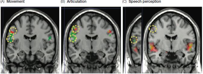
Figure 7.14 fMRI images showing different patterns of activation for lip-related items (red) and tongue-related items (green) across tasks: (A) the movement task involving movement of either lips or tongue; (B) the articulation task involving the production of either /p/ or /t/; and (C) the listening task involving the perception of either /p/ or /t/. (From Pulvermüller et al., 2006, PNAS 103, 7865, © 2006 National Academy of Sciences, USA.)

Results like these, along with the McGurk effect, suggest that information about articulation can be used to inform the perception of speech, even when the listener is doing just that—listening, and not producing speech. But to make the stronger argument that speech perception relies on articulation knowledge, we need to dig a bit deeper.

Does articulation knowledge shape perceptual representations?

If knowledge of articulatory gestures is the foundation on which perceptual categories are built, we would expect to find two things: (1) learning to produce new sounds should have a dramatic effect on learning to perceive them; and (2) the structure of a listener’s perceptual categories—that is, the locations of their phonemic boundaries and their weighting of acoustic cues—should reflect the way in which that listener produces speech sounds.

At first glance, it may seem that perception must precede and drive production, rather than production shaping perception. After all, children’s perceptual capacities seem to be well developed long before they’ve achieved flawless pronunciation. A case in point: At age 3, my daughter pronounced “jingle bells” as “dingle bells.” But if I teased her by proposing we sing a round of “Dingle Bells,” she would become irate and correct me, but ineptly: “Not dingle bells. Dingle bells.” Moreover, as discussed in Chapter 4, in their first 6 months of life, babies show stronger sensitivity to some sound distinctions than adults do—namely, those distinctions that aren’t phonemic in their native language and which adults have learned to collapse into a single sound category—and they do so without having mastered the production of these distinctions. What’s more, certain distinctions, such as the difference between voiced and voiceless sounds, can be perceived by animals that don’t have the physical equipment to produce speech-like sounds (as we saw in Box 7.3). So clearly, some aspects of speech perception are independent of the ability to articulate sounds with any accuracy.

Still, beginning around 5 to 7 months of age, babies spend a lot of time compulsively practicing the sounds of their language (see Box 2.3). In these babbling sessions, which often take place in solitude, babies may be doing more than tuning up the articulatory system for eventual speech. What if they’re also using their mouths as a way to solidify their mental representations of the speech sounds they hear around them? This was exactly the hypothesis of an intriguing study led by Alison Bruderer (2015). Bruderer and her colleagues noted that at 6 months of age, infants in English-speaking households can usually distinguish between certain non-English consonants that are found in a number of Indian languages, focusing on the contrast between /d̪/ and /ɖ/. The dental sound /d̪/ is produced by placing the tongue at the back of the teeth, just in front of the alveolar ridge where the English /d/ is produced. The retroflex sound /ɖ/ is made by curling the tongue tip behind the alveolar ridge so that the bottom side of the tongue touches the roof of the mouth. If babies are mapping these articulatory gestures onto the sounds they’re hearing, and if this mapping is important for perception, then would immobilizing the infants’ tongues affect their ability to distinguish these sounds?

To find out, Bruderer and her colleagues played these sounds to babies who were assigned to one of three groups. One group listened to the sounds while gumming a flat teether that impeded tongue movement; a second group listened with a U-shaped teether that pressed against their teeth but left their tongues free to move; and a third group listened with no foreign objects stuck in their mouths (see Figure 7.15). They found that the second and third groups (who were free to move their tongues) distinguished between the targeted sounds, but the first group of infants, whose tongues were firmly held down by the teether, did not. Whether or not babies could accurately produce the target sounds while babbling, it seems that they were engaging the articulatory system when listening to new speech sounds, and that this affected their performance on the listening task.

Figure 7.15 The teethers used in the infant speech perception study by Bruderer et al. (2015). (A) The flat teether immobilized subjects’ tongues, while (B) the U-shaped gummy teether allow for free movement of the tongue. A third group performed the task with no teether inserted. (From Bruderer et al., 2015, PNAS 112, 13531.)

This study, fascinating as it is, only tests one sound distinction at a single point in time. It’s an open question whether the connection between production and perception would generalize to all sounds at various developmental stages. At 6 months of age, these babies were starting to dedicate serious attention to babbling consonants. What would have happened if the babies were tested, say, at 3 months of age, when they had much less articulatory experience? Or if they were older babies being raised in Hindu-language environments, where they had the benefit of a large amount of auditory exposure to these sounds? Would immobilizing their tongues have any effect on perception under these conditions? And would other sound distinctions, such as voicing distinctions—which can be detected by chinchillas and crickets, among others—be less dependent on articulatory information?

These questions are only beginning to be addressed with infant populations. More work has been done with adults on the connection between production and perception, and here the evidence is somewhat mixed. Some studies have shown that production improves perception. Among these is a study conducted in the Netherlands by Patti Adank and her colleagues (2010), in which participants were exposed to an unfamiliar Dutch accent. Some participants were asked to imitate the accent, whereas other groups were asked to simply listen, repeat the sentence in their own accent, or provide a phonetic transcription of what they’d heard. Only those who had imitated the accent improved in their ability to understand the accented speech. On the other hand, some studies have found no effect of production on perception, or have even found that production gets in the way of learning to perceive new distinctions, as in a study of Spanish speakers trying to learn contrasts between certain sounds that appear in Basque but not in Spanish (Baese-Berk & Samuel, 2016). (In this study, imitating the sounds was a bit less disruptive for perception if the subjects first had some auditory exposure to these sounds without trying to produce them, or of the learning period was extended from two sessions to three.) So, although production seems to support perceptual learning at least some of the time, it’s too soon to be making any hard-and-fast recommendations about exactly when foreign-language-learning software should prompt learners to produce certain sounds.

More evidence for at least partial independence of production and perception comes from studies that take a close look at the category structure of various sounds. If perception relies on representations of how sounds are made, then an individual’s idiosyncratic quirks in how they produce sounds should be reflected in their perception. But several studies show that this is not the case. For example, Amanda Schulz and her colleagues (2012) studied two acoustic cues that help distinguish between voiced and voiceless sounds: VOT and vocal pitch as the consonant is being initiated. VOT is the main cue used by English speakers, but pitch is a significant secondary cue, and individuals differ in how much they rely on each cue to signal the voicing distinction. When Schulz and her colleagues analyzed their participants’ production data, they found a disconnect between cues used for production and perception. In production, people who consistently used VOT to distinguish between voiced and voiceless sounds, with little overlap in VOT between the two categories, were less likely to consistently use pitch as a cue, suggesting that prioritizing VOT came at the expense of using pitch as a cue. But in perception, the relationship between the two cues was entirely different: the more consistent people were in using VOT as a cue, the more likely they were to also use pitch as a cue in perceiving the difference between voiced and voiceless sounds. A similar disconnect between cue weights assigned during perception and production was found in a study examining how native Koreans’ produced and perceived both English and Korean voiced/voiceless sounds (Schertz et al., 2015).

Neuropsychological evidence for the motor theory

The strong version of the motor theory says that perception and production are not merely interconnected, but that perception relies on production knowledge. That is, without being able to access articulatory representations, perception is compromised. The strongest possible evidence for this would be to look at individuals who have trouble accessing articulatory representations due to brain injury or illness, and see whether this has dramatic effects on their ability to perceive speech.

Like the research on the relationship between production and perceptual learning, the results from the neuropsychological literature don’t point to one neat, unambiguous conclusion. The current state of the research is a bit like a jigsaw puzzle whose pieces have been partly assembled, but the connections between clusters of pieces haven’t all been made, and it’s a bit unclear what the overall picture will turn out to look like. If you’d like to see many of the pieces laid out on the table, you can dive into a serious review article (e.g., Skipper et al., 2017). Here, we’ll consider just a few examples to give you a sense of how researchers have been approaching the question.

Alena Stasenko and her colleagues (2015) report a case study of a patient who suffered a stroke that caused damage to his inferior frontal gyrus (IFG), premotor cortex, and primary motor cortex, areas that are involved in articulating speech. As a result, his speech was peppered with pronunciation errors, the most common of which substituted one sound for another (e.g. saying ped instead of bed). He made errors like these even when asked to repeat words or non-words, suggesting that the problem truly was with articulation, rather than a deeper problem with remembering the specific sounds that make up meaningful words. This was confirmed by ultrasound images of his tongue while uttering simple sounds like ada, aba, or aga that revealed his tongue movements to be wildly inconsistent. But when he was asked to state whether pairs like aba-ada or ada-aga were the same or different, his performance was normal, showing the same perceptual boundary between sounds and the same degree of categorical perception as a group of control subjects with no brain damage. (He could also accurately report whether the words in pairs such as pear-bear or bear-bear were the same or different and choose the picture that matched a spoken word like bear from among pictures for similar-sounding words like pear or chair.) But when he was asked to label which sound he’d heard by indicating whether he’d heard aba, ada, or aga, he performed very poorly and showed no sharp boundaries between these sounds.

images LANGUAGE AT LARGE 7.2

How does ventriloquism work?

Good entertainment often bends reality. That’s true in spades for skillful acts of ventriloquism: We know that the words are uttered by the human handler, but we can’t stop ourselves from hearing the dummy “speak” them. So how does this work?

Ventriloquism cashes in on several different illusions. The first of these has to do with perceiving the location of a sound. As is apparent from the McGurk effect, what we “hear” is usually the end result of combining visual and auditory information, whether the cues are about articulation or about the location of a sound in space. In the natural world, visual and auditory cues almost always line up, but since human beings are curious enough to wonder what happens if they don’t, we now know what happens when there’s a disconnect between the two. In a ventriloquist’s act, the lips of the human appear to be still, while the dummy’s mouth flaps in time with the words that are spoken. What happens when your ears are telling you one thing about the location of a sound, and your eyes are telling you something different? It turns out that you believe your eyes. You don’t have to see a ventriloquist to experience this illusion. Have you ever thought about what happens in a movie theater? The sound is coming from speakers placed around the room, but it feels as if spoken words are coming straight out of the mouths of the actors on the screen.

The reason you put more trust in what your eyes are telling you is simply that, most of the time, visual information is a more reliable source of information about an object’s location than auditory information is. But that can change in a situation where the visual cues become fuzzy or indistinct—in that case, you’d likely depend more on sound to figure out an object’s location in space. It’s also possible that the location illusion is affected somewhat by where you’re directing your visual attention. If you look at YouTube clips of ventriloquist acts, you might notice that the dummy is usually designed to draw more visual attention than the human—the dummy often wears bright clothing, has humorous facial features, and is very animated in its movements, while the human tends to blend into the background by wearing nondescript clothing and limiting movements of both the face and body while the dummy is “speaking.”

The second kind of illusion deals with the actual sounds of speech and how they’re interpreted. Ventriloquists manage to speak without moving their lips, so how is it that they’re able to produce the full range of speech sounds? The answer is that they don’t; to some extent, they can rely on us as hearers to hear what we expect to hear rather than what’s really there.

Ventriloquists speak with their lips still and partly open, which nevertheless allows them to make many speech sounds by controlling the shape and movement of the tongue behind the lips in a way that’s not visible. But sounds made by moving the lips—like /b/, /p/, /w/, /m/, /v/, and /f/—are problematic. To some extent, the ventriloquist can write a script that avoids words containing these sounds, but when absolutely necessary, these labial sounds can be replaced by other similar-sounding phonemes. For example, /f/ might be replaced by /θ/ (the first sound in think), and /m/ by the similar-sounding /ŋ/in sing. We’ve already seen from the Ganong effect and phoneme restoration effect that the sounds we think we hear depend to some extent on the sounds that we expect to hear in a particular word. Ventriloquism takes full advantage of this.

Based on some of the results that we’ve talked about with these particular auditory illusions, we should also be in a position to offer some scientifically grounded advice to an aspiring ventriloquist. For example, remember the Ganong effect, in which a sound was perceived in such a way as to be consistent with the rest of the word. If you want your hearer to perceptually morph a d into a b sound, best to use the sound in a word where it wouldn’t make sense as a d. (For example, in dest, but not in dust when it’s intended to be heard as bust.) Remember also that the effect of the surrounding word was strongest when the sound itself was ambiguous—clear examples of sounds that made no sense in the words they were embedded in (for example, dest) were just perceived as mispronunciations. This suggests that you can’t simply throw in a clear-sounding d and expect it to be heard as a b sound, even if the word makes no sense with a d sound. For this reason, ventriloquist manuals usually suggest altering the substituted sounds in some way. For instance, one way to make a d sound slightly more like a b sound is to pronounce it by placing the tongue against the teeth rather than in its usual position on the ridge behind the teeth. It takes some practice to distort certain sounds so that they become more acoustically similar to the intended labial sounds.

The phoneme restoration effect showed that even quite garbled sounds can be reinterpreted as specific phonemes, and that the illusion is especially strong with long words that have few similar-sounding competitors, and with words that are generally quite predictable in context. In other words, the more strongly activated the word is, the stronger an impact it’s likely to have on how people perceive the sounds within it. It seems to make sense, then, that words that contain substituted sounds should be ones that are likely to be strongly activated in the context.

Once you start seeing how this genre of entertainment fits neatly with a model of normal, everyday speech perception, it might be hard to stop making the connections. In fact, you might even be tempted to make specific predictions about best ventriloquist practices and then put them to rigorous empirical tests by adapting some of the experimental approaches you’ve learned about here.

Problems with articulation are also experienced by people who have more general disorders of movement, such as Parkinson’s disease (a degenerative disease of the central nervous system that affects the motor system) and cerebral palsy (a movement disorder that results from brain damage at birth or in early childhood). Do the resulting difficulties with pronouncing words crisply and accurately affect how these individuals perceive or represent the sounds of speech? A longitudinal study led by Marieke Peeters (2009) found a connection between speech production abilities in children with cerebral palsy and certain sound-based skills. Specifically, they found that children’s pronunciation skills at ages 5 and 6 predicted their performance at age 7 on tasks that required an awareness of the sound structure of words—for example, identifying which of several words began with the same sound or whether two words rhymed or not. (Speech production abilities also predicted the children’s success at decoding written words—stay tuned for the Digging Deeper section to see how reading skills are connected to mental representations of sounds.) But the connection was much weaker between production ability and the ability to distinguish speech sounds by saying whether two similar words were identical. These results echo those of Alena Stasenko and her colleagues in that making perceptual distinctions between sounds was less affected by pronunciation problems than the ability to consciously manipulate abstract representations of sounds.

There’s a neat logic to the strategy of finding naturally occurring problems with articulation and studying their effects on perception. But, as you saw in Chapter 3, brain damage often affects many regions, not just those that researchers happen to be interested in studying. This can leave some doubt as to whether it is damage to the motor system that is driving the perceptual difficulties, or damage elsewhere. (For example, patients with Parkinson’s may also experience cognitive problems with attention and working memory, and some children with cerebral palsy also have intellectual disabilities.) Current technology offers a workaround to this problem: It is now possible to recruit healthy, willing participants into lab experiments, and temporarily disable specific brain regions using a technique known as transcranial magnetic stimulation (TMS). To apply TMS, researchers place a magnetic field generator (called a “coil”) near a person’s head to create electric current in a small, targeted region of the brain. This causes random firing in a population of neurons, which essentially creates neural noise that can disrupt the normal functioning of that area of the brain. The effects of TMS are immediate and dramatic. When brief pulses of magnetic stimulation are delivered at low frequencies over a sustained period (say, 15 minutes), this can affect the functioning of the targeted brain area for a similar length of time after TMS has been applied.

This technique offers something that brain science pioneers like Paul Broca and Karl Wernicke probably could not have imagined in their wildest dreams—a way to create temporary “lesions” in the brain and observe their effects. And it’s especially handy for studying the link between articulatory knowledge and speech perception because it’s actually possible to locate and target specific areas of the brain that control articulators like the lips and tongue. TMS allows researchers to do at a neural level what Alison Bruderer and her colleagues did by physically restraining the action of babies’ tongues. In other words, it allows them to ask whether speech perception can be disrupted not just by preventing certain articulators from moving, but by preventing people from thinking about the movement of their articulators, even unconsciously.

Riikka Möttönen and Kate Watkins (2009) published an elegant study along this line of inquiry. Their strategy was to apply TMS to a region in the motor cortex that controls lips movements and see whether this affected their subjects’ performance on categorical perception tests involving the contrast between /ba/ and /da/. These sounds are differentiated by their place of articulation, with /ba/ involving the lips and /da/ involving the tongue against the roof of the mouth. If motor representations play a key role in this type of perception, then disrupting the neural processing of lip-related movement should affect the ability to make this distinction. On the other hand, it shouldn’t make a difference to the ability to distinguish between /da/ and /ga/, because neither of these sounds involve the lips. This is exactly what Möttönen and Watkins found: when subjects heard slightly varying examples of /ba/ or /da/ (or /da/ and /ga/) before receiving magnetic stimulation, they showed the typical pattern of categorical perception, in which slightly different sounds were much less likely to be perceived as different when they were both members of the same category than when they were members of different categories. But after the application of TMS, subjects showed a more continuous pattern of perception for /ba/ versus /da/, with a less sharp category boundary imposed on the sounds. But the perception of /da/ versus /ga/ was not affected by TMS applied to the lip region of the motor cortex.

This is certainly a clever study with compelling results, but some researchers have questioned exactly what it means for normal speech perception that takes place outside of the lab and in real time. As you saw in Section 7.1, true categorical perception is not found in some tasks even when people’s brains aren’t being zapped by TMS. Just how important, then, are gestural representations for the daily task of speech perception? Researchers still disagree about this, with some arguing that articulatory knowledge comes into play most heavily when people are asked to consciously manipulate abstract categories of sound or to understand speech in especially difficult situations—for example, when the environment is noisy or the speech sounds are especially unfamiliar.

It’s clear that there are at least some intimate connections between articulation knowledge and speech perception, though researchers are still working out what these connections are and when they come into play. It’s also evident that perception doesn’t rely crucially on motor representations. If these representations are absent or made less accessible, the effects on perception aren’t catastrophic, suggesting that the perceptual system can do much of its work by relying on acoustic cues alone. This lack of a strong, unambiguous conclusion may seem unsatisfying, but it’s actually well aligned with our emerging understanding of how the brain works. Language functioning is not to be found in a specific region of the brain, or even within one neatly organized brain network; instead, it’s distributed among a number of different networks that perform different but partially overlapping functions—and whose performance may change as a person ages (see Box 7.6). This complexity is inherent in something as basic as the act of perceiving the basic units of language.

GO TO

oup.com/us/sedivy2e

images BOX 7.6

What happens to speech perception as you age?

Many people find it harder and harder to follow conversations as they get older. Their younger relatives may urge them to just get a hearing aid already. This may not always solve the problem. This is because loss of hearing isn’t the only relevant factor. Aging is also associated with a number of changes in the brain that affect the understanding of speech. As you’ve seen in this chapter, processing speech sounds involves a lot of mental activity beyond being able to accurately detect the incoming acoustic signal. So, merely turning up the volume isn’t always going to help, or if it does, it’s unlikely to completely fix the problem.

Many of the difficulties that older adults have with speech perception can’t be predicted by hearing tests (for a review, see Pichora-Fuller, 2003). Even older adults with normal hearing are worse than younger people at understanding speech that is very fast or that takes place in a noisy environment. They may have more trouble identifying individual voices, which could affect their ability to separate the voice of the person they’re listening to from other voices in the background or to reap the benefits of talker adaptation. Changes in attention make it harder to suppress irrelevant information. Generally, the processing of auditory information (both speech and non-speech) slows down. And older people who show no decline in their ability to hear tones at various frequencies and volumes might still show impairments in the processing of temporal auditory information—that is, information about the timing of auditory events. This would reduce their ability to use important acoustic cues like VOT or vowel durations. All of these factors can add up to make speech perception extra work for older people—even without throwing in the very common problem of hearing loss.

The fact that speech perception relies on a multiplicity of cues provides some insurance against age-related changes, allowing for abilities that are intact to compensate for less reliable ones. Visual cues can be especially useful for those who have trouble processing auditory information, whether due to hearing loss or other factors. In a study led by Kaoru Sekiyama (2014), adults age 60 to 65 with normal hearing were found to have a stronger McGurk illusion than participants between the ages of 19 and 21, suggesting that the older adults placed more importance on visual articulatory information than the younger group. They also took longer to identify the target syllables when they heard them but did not see any accompanying video. However, they were no slower than their younger counterparts to identify syllables based only on the visual information in the video. The authors suggest that at some point, the ability to process auditory information declines more sharply than the ability to process visual articulatory information, leading to a shift in the cues used for speech understanding.

It’s a cruel irony, then, that age can also lead to a decline in lip-reading ability, despite the fact that older people have a greater need for visual cues. In a study that compared the performance of younger (average age of 20) and older people (average age of 76—somewhat older than those in Sekiyama study), the poorer lip-reading performance of the older group was linked to worse performance on tests of working memory and tasks that measured processing speed in response to visual stimuli (such as the speed of deciding whether a string of letters was a real word or not). And there’s even a hint in the research literature that hearing loss itself may contribute to a decoupling of brain regions that process auditory and motor information. This is the argument advanced by Muriel Panouillères and Rikka Möttönen (2017), who used TMS to study the excitability of the region of the motor cortex that controls the tongue in older and younger participants as they listened to speech. They found reduced activity for older adults (average age of 68) who had hearing loss, but participants of the same age without hearing loss showed the same responsiveness as younger subjects (average age of 21).

These studies make it clear why many older adults feel that the entire world is designed for the perceptual profiles of younger people—what with the loud music in public spaces, sleek surfaces in restaurants that bounce sound in all directions, and the rapid-fire dialogue in many movies and TV shows. Hearing aids—or even technology that can dynamically slow down speech—can help to some extent. But so could more intelligent design decisions that take into account the age and perceptual traits of a target market.

DIGGING DEEPER

The connection between speech perception and dyslexia

Developmental dyslexia is a common learning disability that leads to difficulties in learning to read, but no obvious problems with spoken language or other learning problems (though people with dyslexia are more likely than the general population to also have other problems, such as specific language impairment). Dyslexia is known to have a strong hereditary basis, and a number of candidate genes have been identified as probably playing a role. So, should we conclude that dyslexia is a selective impairment of genes that are responsible for reading?

Here’s where that idea has trouble getting off the ground: writing is a fairly recent invention. As a species, we’ve only been reading and writing for several thousand years, a much shorter time than we’ve been speaking. And while speaking (or signing) is universal among humans, many societies or social groups currently exist without feeling the need to put things in writing. Moreover, even within societies that have had writing systems for a long time, it’s only very recently that literacy has become common within the general population rather than being a skill learned only by a few. It is highly implausible that, in such a short time, we could have evolved genes dedicated to the mastery of this recent, non-universal, elite cultural tool. What’s more, there’s no evidence that people who come from societies (and therefore gene pools) with low literacy rates have any greater difficulty in learning to read than those who come from countries where a large segment of the population has been reading for centuries. So, what to make of the connection between genes and reading?

A plausible explanation is that reading relies on genes that didn’t develop specifically for reading, but that the affected genes contribute to a skill that turns out to be highly relevant for reading. A closer look at the abilities of people with dyslexia has turned up a consistent sticking point: difficulty with phonemic awareness, or the ability to consciously analyze strings of sounds into their subparts (e.g., Snowling, 2000). For instance, many dyslexics have trouble with requests and questions like these:

Which word has a different first sound: beetle, bat, chair, or bust?

Say catch. Now say it again, but don’t say the “k” sound.

Here is a picture of a desk. Now finish the word for me: des__.

It’s easy to see how trouble in consciously isolating individual sounds from longer strings would be a problem for learning to read (at least in a writing system like that of English)—the whole enterprise hinges on matching up individual sounds with visual symbols. In fact, across various languages, research has shown strong evidence that phonological awareness is highly predictive of later reading ability.

Many researchers support the idea that dyslexia, along with its attendant difficulty with phonemic awareness, has its roots in underlying problems with speech perception and the development of sound categories. These problems are too subtle to cause noticeable issues with spoken language. As you’ve seen, speech understanding draws on multiple acoustic cues and variously detailed (or abstract) levels of representation, which may make the whole system somewhat resilient in the face of any specific deficits. Such resilience may even be due to evolutionary adaptation, ensuring that subtle genetic variation won’t have a catastrophic effect on our ability to understand language. But written language is clearly an artificial linguistic device, much like a prosthetic limb attached to our organic, biological parts. It takes concerted effort to learn to use it effortlessly, and the evidence suggests that it’s especially vulnerable to even slight disruptions in our mental representation of sounds.

A number of studies have found that people with dyslexia (or who are at genetic risk for dyslexia) perform unusually on tests of categorical perception, as noted by Mark Noordenbos and Willy Serniclaes (2015), who analyzed the results of 36 such studies. Specifically, dyslexic participants tend not to make as sharp a distinction as others between similar sounds that straddle phoneme boundaries, and conversely, where control subjects ignore differences between similar sounds within a phonemic category, dyslexic participants register these differences to a greater degree. That is, they tend to consider two variants of /p/, for example, to be more different from each other than most people would, whereas the differences between /p/ and /b/ are somewhat blurred. In Section 7.1, you saw arguments that, even for typical listeners, the actual perception of speech is not categorical in nature—that is, listeners show quite a bit of sensitivity to small within-category differences in the course of natural word recognition. But more abstract sound categories can normally be accessed and manipulated when the task calls for it, such as when people have to make a conscious decision about which type of sound they’re hearing. This is exactly the kind of mental work that’s involved in reading and writing—the sounds of speech have to be labeled and linked up with a corresponding symbol. The usefulness of drawing sharp acoustic boundaries between the things written as P and those written as B are pretty clear: if the differences between all /b/ sounds are downplayed mentally, so that they’re considered examples of the same kind of thing—much as at some level, we think of an armchair and a desk chair as examples of the same kind of thing—then the task of labeling is easier. But if various /b/ sounds are represented as separate kinds of things, then it’s less transparent why they’re all connected to the same symbol.

Other evidence supports the notion that people with dyslexia are less able to distinguish and categorize sounds in a way that is especially useful for written language. Section 7.3 discussed the process of talker adaptation, which allows us to better understand speech from a talker we are familiar with. Adaptation occurs because we learn to pay more attention to the cues that are most useful for distinguishing between sound categories for that person, and less attention to cues are less useful. In a study led by Tyler Perrachione (2011), dyslexic people showed less adaptation to talkers’ voices, suggesting that they had trouble tuning their attention in this way. Again, the impact on everyday speech perception might be subtle. If you don’t have dyslexia, you might imagine what the speech world would sound like if familiar voices didn’t sound, well, familiar. You could still understand what these voices were saying, but it would take just a bit more effort, as if you were constantly hearing everyone’s voice for the first time (and perhaps it would also be a bit like listening to a new accent for the first time, without the benefit of previous experience with it).

Do such subtle glitches in speech perception really lead to the dramatic problems that dyslexic people have with learning to read and write? Establishing the causal connection turns out to be a bit tricky. This is because the relationship between literacy and speech perception also goes the other way—that is, there is clear evidence that learning to read reorganizes the way in which we mentally represent speech sounds. For example, phonemic awareness may be an important predictor of reading ability, but it’s also a result of learning to read. It may seem completely natural to you to think of the word cat as consisting of three distinct sounds, the first of which is identical to cone. But phonemic awareness is not something that spontaneously emerges at some point in development. Surprisingly, even adults who are not literate have quite a bit of trouble with simple tests of phonemic awareness. (They do much better on tests where they’re asked to identify or manipulate syllables than single phonemes, suggesting that breaking speech down into phonemic units may not be as important for daily spoken language as we might think.) But illiterate adults who learn to read go on to develop better phonemic awareness, showing that this skill is more closely tied to experience with written language than it is to age or spontaneous neural development (Morais et al., 1986).

Performance on categorical perception tests is also responsive to reading experience. In one study (Noordenbos et al., 2012), children who were at risk for dyslexia showed somewhat blurry sharp phonemic boundaries when they were in kindergarten, before they learned to read. But in first grade, 6 months after starting formal reading instruction in school, this difference had completely disappeared and their performance on categorical perception tests was indistinguishable from that of their peers.

Results like these are fascinating, because they suggest that reading re-shapes our mental constructs of speech sounds. If reading is like a prosthetic limb, then it’s one that becomes so embedded with the rest of the body that it alters the biology of the “natural” parts to which it attaches. But these results also make it difficult to draw clear conclusions about the underlying causes of dyslexia. While it’s certainly plausible that deficiencies in the categorization of speech sounds could lead to problems with written language, we can’t rule out another explanation: whatever the underlying causes of dyslexia, people who have it are likely to read much less as a result, or read less fluently. If reading experience boosts phonological representations, and people with dyslexia read less (or read less well), then they would naturally have impaired phonological representations compared to strong readers. Of course, the matter is made more complicated by the fact that the cause–effect relationship may well run in both directions at once.

To disentangle all of this, it’s important for cross-sectional studies—that is, studies that test and compare different groups at a single point in time—to include the right groups as comparisons. In addition to testing participants with and without dyslexia, the effect of literacy should be controlled for, so that if older literate subjects are being tested, then there needs to be a non-literate group as well (this could pose some practical problems in studies of adults in countries that have a very high literacy rate). An even better solution would be to conduct careful longitudinal studies, in which the same group or multiple groups are studied over time, ideally before and after learning to read, thereby allowing for a clearer separation of the predictors versus consequences of reading ability.

A number of such longitudinal studies have been carried out to date, and there does seem to be evidence for an underlying causal role of speech perception abnormalities. For example, Bart Boets and his colleagues (2011) tracked children from kindergarten to third grade and found that those who were diagnosed with dyslexia in third grade had shown early impaired performance in perceiving speech mixed with noise, along with other auditory deficiencies. In fact, these emerged as strong predictors of reading ability even when other reading-specific skills, like phonemic awareness and the ability to recognize letters, was controlled for. One of the most dramatic longitudinal demonstrations comes from a study published by Dennis Molfese (2000), in which 186 children were followed from birth to age 8. Molfese first tested EEG responses to the contrasting syllables /bi/ and /gi/ in his subjects within 36 hours after birth, and every year thereafter. Over time, these children were classified into three groups: (1) those with dyslexia, who had poor scores in reading, but not low IQ scores; (2) poor readers who also had low IQ scores; and (3) children who had typical scores on both tests. Even at birth, the EEG responses to speech sounds differed among these three groups (see Figure 7.16).

We need much more in the way of detailed research looking at various components of speech perception, their connection to reading skills, and the extent to which they are affected by reading experience. But these longitudinal studies provide some of the strongest evidence we have that dyslexia emerges out of individual differences in speech processing. Moreover, they contradict the claims made in some educational circles that dyslexia is not a “real” diagnosis, but a cover for poor pedagogy or lazy study habits. And they also suggest that, much as reading may feel instinctive and “natural” to voracious, fluent readers, in reality it’s a somewhat fragile skill that requires a restructuring of mental representations. Unfortunately, it appears that it can be derailed by genetic variations that otherwise leave few scars on spoken language functioning.

Figure 7.16 Event-related potentials (ERPs) recorded over left and right frontal regions from three groups of infants at birth in response to the syllable /bi/. Different patterns of activity were apparent for infants who would later be categorized as dyslexic (red line), as poor readers who did not meet criteria for dyslexia (yellow line), or as typically developing controls (blue line). (From Molfese, 2000, Brain Lang. 72, 238.)