CIVIL ENGINEERING SYSTEMS ANALYSIS

This chapter goes beyond the basic concepts learned in Chapter 4 and uses them on practical applications. In this chapter, we learn two important concepts: estimation and prediction. As we will see, they are both interrelated. Estimation is the science of calibrating an equation that provides a representation of the real world containing only those elements deemed important given their capability to capture the phenomena being modelled. Prediction is the art of forecasting future states or values of a phenomenon. This typically has the purpose of making decisions to change the future. Prediction typically uses calibrated systems (estimation) along with some additional factors.

5.2 Estimation

Estimation is the ability to encapsulate a phenomenon mathematically. To be able to estimate, we need to create a functional form with at least one equation capable of capturing the nature of the phenomenon using measurable (observable) responses and factors that contribute to explain it. This sounds a lot like a regression analysis, and in many cases researchers could be tempted to run a regression and use it for estimation. However, you must note that a regression does not have the ability to capture the nature of the phenomenon in the relationships between the factors and the response. You could, however, prepare a linear regression to gain quick understanding of the relationship between observable or measurable factors and a response. However, you need to move ahead and estimate a mathematical representation of the factors and their contribution to the response. For this, we need to follow three steps:

1. Identify what elements play an important role on it.

2. Identify the functional form of the relationship between the response(s) and the factors.

3. Calibrate the mathematical expression.

Following these three steps will lead you to identify a functional form that contains a good representation of the nature of the phenomenon and the factors that play a role. You will use coefficients to calibrate the role of the factors and to adjust the mechanism(s) to match real-life observations.

After step 2, that is, when you obtain a representation of the system, you proceed to step 3 to calibrate the coefficients. This is however a tricky one. When the functional form is only one equation and you need to estimate several coefficients (unknowns) with an observed response per combination of factors, your only choice is to run a regression to estimate the values of the coefficients.

When you have a system of equations that predict the same number of indicators as unknown coefficients, then you could follow an iterative process to estimate them. In this case, it is typical that you would have to develop a strategy to calibrate the values in order to replicate those indicators (responses) to match their observed values.

Typically, you may need to iterate the value of the variables until you are able to replicate observed responses. For the remaining of this section, we concentrate our attention to an example.

5.2.1 Worked Example for Pavement Deterioration

This section describes a worked example that estimates pavement deterioration in the form of international roughness index (IRI). This index measures the total amount of vertical variation of a dumping system of a vehicle rolling through a road. The smoother the ride, the less vertical oscillations the system will experience. Vertical variations are measured from rest, and they all accumulate whether the tire moves up or down; it is like using the absolute value of the deviations.

The response for this example is an indication of the condition of the pavement, and a brand new pavement should be equivalent to a surface that has zero imperfections; hence, the ride should be very smooth and the value of IRI should be close to zero. As time passes, the layers underneath the pavement suffer from the effects of the weather and lose strength; this leads to loss of support which translates into deformations of the surface.

Thicker pavements are commonly associated to higher strength, however this must be contrasted to the number of heavy trucks using the pavement every year and environmental factors: the water in the subgrade soil could freeze and heave and certain types of soils swell with the presence of water.

The previous paragraph provides us with a description of factors (elements) that contribute to explain the selected response. Now, we need to move through the steps of the estimation. The first step is to identify the elements that play a role, and this signifies the need to have one measurable indicator per element. So here is our list of elements: truck traffic, subgrade soil and pavement layer strength and weather (water). As it turns out, we could estimate the number of equivalent single axles (ESALs) of a given weight (80 kN or 18,000 lb) per year from traffic counts.

There is an expression called structural number developed by the American Association of State, Highway and Transport Officials that combines the thickness and quality of materials of the pavement into one that provides an indication of how strong the pavement is. Finally, there is an expression called Thornthwaite Moisture Index which reflects the weather of a given region by estimating its degree of water arriving to the soil. Table 5.1 shows the process of identification of factors and response we are trying to model.

The next step is to identify the nature of the relationship between the factors and the response. First, we need to think of the response moving in one particular direction, which is typically chosen as the undesired direction; in this case, an increase in deterioration is also an increase in IRI (Table 5.1).

Next, we identify the movement on each variable that produces an incremental effect on the response. For the first factor, an increase in the number of trucks will damage the pavement and so it will deteriorate more. So we could identify a direct response.

For us, a direct response signifies that an increase on the factor returns an increase on the response. For the second factor, an increase in pavement strength translates into a decrease in deterioration; the stronger the pavement, the less it deteriorates. We will call this type of relationship inverse. Finally, the more water reaching the pavement, the more it will deteriorate (from the effects of swelling and heaving), so the relationship in this case is direct as well.

To complete step 2, we simply associate direct relationships with a multiplicative effect and inverse effects with a division effect. So our relationship so far could take on a primitive functional form shown by the following equation:

TABLE 5.1
Factors That Contribute to Pavement Deterioration

Element	Description	Indicator	Relationship
Response	Deterioration	IRI	Incremental
Factor 1	Truck traffic	ESALs	Direct
Factor 2	Pavement strength	SN	Inverse
Factor 3	Presence of water	m-index	Direct

$I R I = \frac{(m - i n d e x) (E S A L s)}{S N}$

At this stage, we have completed step 2; however, we are presuming that all (direct and inverse) relationships are linear, which is somewhat a very strong assumption. So in order to relax this assumption, we introduce coefficients to raise each element. The calibration that proceeds on step 3 will confirm (coefficient = 1) whether or not the relationships were linear. Our functional form takes now the following form:

$I R I = \frac{{(m - i n d e x)}^{α} {(E S A L s)}^{β}}{S N^{δ}}$

Notice that the response remains intact, and we do not apply any coefficient to it. Now, we concentrate on step 3. We need to calibrate the coefficients α, β and δ to replicate the response. Table 5.2 contains a sample of observations that we will use for this purpose.

TABLE 5.2
Sample Data Deterioration

*IRI*	*ESALs*	*SNC*	m
0.18	60,000	3.96	0.04
0.45	122,000	3.96	0.06
0.67	186,000	3.96	0.08
0.54	251,000	3.96	0.04
0.95	317,000	3.96	0.06
1.08	384,000	3.96	0.08
0.83	454,000	3.96	0.04
1.46	524,000	3.96	0.06
1.48	596,000	3.96	0.08
1.17	669,000	3.96	0.04
1.89	743,000	3.96	0.06
1.96	819,000	3.96	0.08
0.88	897,000	3.96	0.02
1.82	976,000	3.96	0.04
1.67	1,057,000	3.96	0.05
2.66	1,139,000	3.96	0.07
1.30	1,223,000	3.96	0.02
1.43	1,309,000	3.96	0.03
2.40	1,396,000	3.96	0.05
2.39	1,486,000	3.96	0.04

First, notice that we have developed one equation only. You have three coefficients (unknowns) and only one response, with one observation of the response per set of observed levels of the factors. So, we will proceed to run an ordinary least-square optimization to obtain the values of α, β and δ that minimize square differences between predicted and observed levels of IRI.

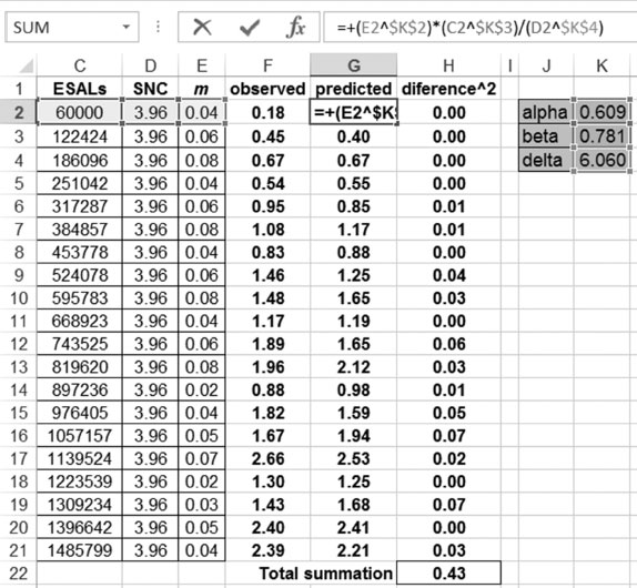
We can do this in Excel. First, we need to transfer the data from Table 5.2 into an Excel spreadsheet. Then we use the functional form created on step 2. Three additional cells in Excel will be used to contain the values of the coefficients α, β and δ. Then an additional column called predicted is added into Excel, and its value is coded to match the functional form along with the value of the unknown coefficients as shown in Figure 5.1.

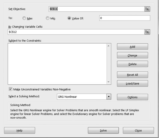
Finally, the square difference between the observed value of IRI and the predicted value (using the functional form) is added into the spreadsheet. The total summation of the square differences becomes the objective of our optimization. There are however no constraints. As you can see, the problem is an unconstrained optimization, and the coefficients could take on any value.

FIGURE 5.1
Excel set-up.

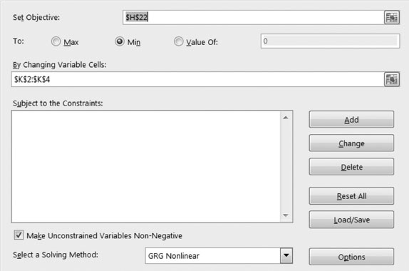
FIGURE 5.2
Excel’s add-in solver set-up.

The reader must notice that before solving I set up the values of the coefficients to zero (you could have used the value of one); however, using zero allows the solver to depart from the non-contribution perspective, that is, a coefficient with a value of zero will have no contribution on the observed response.

Figure 5.1 shows the Excel set-up and the calibrated values from the optimization. Figure 5.2 shows the actual set-up on Excel’s add-in solver used to find the calibrated values.

If you ever move into graduate school, then you will possibly learn how to develop systems of equations that are interrelated in which you could follow an iterative strategy to calibrate the coefficients (I do, however, present a couple of examples in Chapter 6). Deep understanding through years of research is typically devoted to develop such systems. Often, the equations you learn throughout your undergrad degree are the product of years of research, and as you will soon realize, the values of any constants on the equations are nothing more than calibrated values.

5.2.2 Example of Road Safety

We look into an example of road safety in which we want to build a functional form to estimate the contribution of several factors such as the number of lanes, density of intersections and others on collisions. Availability of data varies from government to government.

The three previous steps are repeated. First, we identify that there are many factors all related to collisions, traffic volume in the form of annual average daily traffic (AADT), number of lanes (x₁), density of intersections (x₂), width of shoulder (x₃) and radius of curvature(x₄).

We will not worry about step 1, that is, we will let the coefficients of our regression give us the indication of whether a factor has a direct (positive) or an inverse (negative) contribution to explain the response. For step 2, we will borrow the classical functional form shown in the following equation:

$y = (A A D T^{α}) e^{b_{1} x_{1} + \dots + b_{n} x_{n}}$

To conduct a linear regression, we need to warrant having a linear form, so we will apply natural logarithm on both sides of this expression, obtaining

$ln y = α (\ln A A D T) + b_{1} x_{1} + \dots + b_{n} x_{n}$

If you simply think of lnAADT as a variable (say x₀) and the response lny as a typical response (call it r), then the entire expression collapses into a linear form:

$r = α (x_{0}) + b_{1} x_{1} + \dots + b_{n} x_{n}$

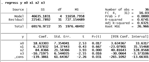
Given the fact that we have a linear expression, we can use a linear regression to estimate the value of the coefficients. For this, we turn our attention to STATA^®. As learned before (Chapter 4), we can run a linear regression by writing the following in the command line: regress rx₁x₂x₃ …. Table 5.3 shows the observations used in this example.

The next step is to transfer the data from Excel (or any other database you maybe using) to STATA. The results from STATA are shown in Figure 5.3. As you can see, the number of lanes does not play a role on the explanation of collisions. The higher the traffic volume (AADT) and the higher the density of intersections, the more collisions we observe (both coefficients are positive), and the wider the shoulder, the less collisions we observe. The reader needs to remember that at a confidence of 95%, the corresponding p-values must be smaller or equal to 0.05. In this case, the p-value for x₁ goes way beyond such point and deems the number of lanes insignificant.

5.2.3 Estimation of Explanatory Power Standardized Beta Coefficients

This section presents the case of estimation when the explanatory power of the factors is needed for a specific purpose. If we use a simple regression to obtain the values of each beta, we will obtain one interpretation for traffic volume and other interpretations for the rest of the causal factors. Whenever you need to compare the contribution of elements to explain a response, you will need to standardize all the values on your database. This is achieved by taking each observation for a given factor, subtracting from it the mean of the factor and dividing by the standard deviation of the given factor under consideration.

TABLE 5.3
Sample Data Road Safety

y	x₀	x₁	x₂	x₃
28	8.78	2	0.5	0
6	8.77	2	0.17	2.67
22	8.78	2	0.5	0
133	9.23	1	0.63	1.13
162	9.13	2	0.8	0.47
2	8.28	2	0	1.80
5	8.28	2	0.17	0.45
23	9.17	2	0.17	2.5
119	9.11	3	0.7	0
162	9.08	3	0.85	0
46	8.27	3	0.43	1.89
3	8.03	2	0	1.5
13	8	2	0	1
8	8.2	2	0	0.45
5	8.2	2	0.33	1
20	8.14	2	0.5	1.4
17	8.3	2	0.5	2.33
2	8.46	2	0.17	2.23
3	8.47	2	0	1.7
3	8	2	0	2
11	8.05	2	0	1.5
3	8.05	2	0	2
12	8.04	2	0.71	0.86
7	6.9	2	0.17	0.65
9	6.9	2	0	0.65
3	7.97	2	0	0
2	7.97	2	0	1.05
2	7.97	2	0	0.53
3	7.78	2	0.33	1.42
4	7.33	2	0	0
2	7.13	2	0.17	1.25
6	7.13	2	0.33	0.93
3	7.14	2	0.33	1.25
2	6.92	2	0	1.2
6	6.23	2	0	0.6
6	6.77	2	0	1.03

FIGURE 5.3
STATA^® linear regression.

Once you have done this, you can run a regression and obtain the standardized beta coefficients for each factor. This coefficients will read as the amount of variation that you need on each factor alone to produce a variation of 1 standard deviation on the response.

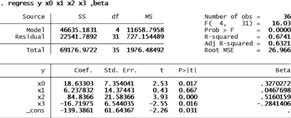
There is a built-in option on STATA to obtain the standardized beta coefficients automatically. In the command line after, you simply add the command beta after you specify the traditional regression: regressyx₁x₂x₃, beta.

The obtained values allow you to compare the explanatory power of each factor to explain the response. You can divide two beta coefficients and directly estimate how many more times one factor is capable of explaining the response. At this stage, you are probably wondering why and how you would ever use that. Here, I present an example that has been further addressed elsewhere by myself.

For instance, think of the warrant system for roadway lighting. The recommended coefficients used to make decisions for the provision (or not) of lighting are not calibrated, and for this reason they do not always work in the proper way when you sue this system. To make them work, you need to change them in such a way that their values reflect reductions in road collisions. This approach is called evidence based, and the aim is to have values that would be learned from crash history, that is, we will calibrate the scores of the warrant to values that warrant lighting when it will counteract night-time collisions.

For the calibration, we need to look into the explanatory power of each road deficiency to explain night-time collisions. That is, we have a series of geometric, operational and built environment elements that we can measure, and certain values of this elements represent higher degrees of deficiency of the road and then contribute to night-time collisions.

For instance, think of the width of the shoulder or width of the lane. If the shoulder is less than 2.5 m or the lane is less than 3.6, we step into deficient values. A lane of 2.5 m is so much more deficient than a lane of 3 m, so they could be blamed for producing collisions in dark circumstances at night when visibility is reduced and the driver expects a standard width lane (or shoulder that fully protects a stop vehicle). In a similar manner, we think of lighting as a countermeasure to help reduce the frequency and severity of collisions at night-time, counteracting the deficiencies found in other elements, that is, improving visibility.

To calibrate, we need to take the explanatory power of each element and use it to explain observed collisions. I present a very small database (in real cases, it contains hundreds, if not thousands, of segments) to illustrate this problem. A final word is important: when you obtain the standardized coefficients, you simply need to normalize them and rescale them in order to obtain the new values of the lighting warrant grid scores.

Table 5.3 (in the previous section) contains the information we will use for this example. We direct our attention to the STATA output once we include the beta command. Figure 5.4 illustrates the STATA output for the same example.

The contribution of x₀ (lnAADT) to explain the response is quite close (1.15 times) to that of x₃ (shoulder width), for the density of intersections (x₂) is about 1.8 times that of the width of the shoulder. With these values, it is easier to add them and obtain weights for their contribution, which will then be translated into scores. Table 5.4 shows the calculation of the scores. It is important to mention that the weights are multiplied by a factor of 20 in order to obtain scores. This number comes from the fact that the total combined contribution of the factors must add up to 20 and then is multiplied by another amount called classification points that we will not change ourselves.

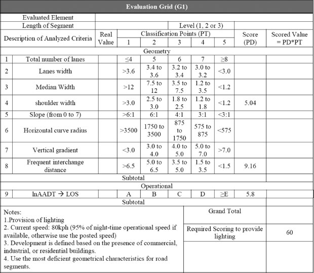
Figure 5.5 shows the finally calibrated grid which only uses those significant elements in order to make decisions for the provision of roadway lighting. The reader can search for the original grid score for highways (called G1) and realize that what we have done is simply the estimation of the explanatory contribution of each factor to explain collisions. We have used a standardized form in order to be able to express all contributions in common units. After this, the only remaining task is to modify the grid to contain only the significant factors, and the original values are changed to those estimated from the contribution to explain collisions, and hence, we end up with an evidence-based approach.

FIGURE 5.4
Standardized betas.

TABLE 5.4
Calibration of Scores

Element	Standardized Beta	Weight	Score
lnAADT (x₀)	0.327	0.290	5.80
Density intersection (x₂)	0.516	0.458	9.16
Shoulder width (x₃)	−0.284	0.252	5.04

FIGURE 5.5
Calibrated scores for roadway lighting.

Some warnings are important to the reader. First, the reader must remember that a correlation analysis must be performed before selecting the causal factors that will be used for the analysis. Correlation typically takes the form of a matrix that identifies colinearities between factors and the response or simply between factors themselves, when the value of colinearity is high that signifies that the value should be dropped from the analysis.

The other element the reader must bear in mind is that more data and more elements should be used; however, sometimes data are not available and yet decisions need to be made. In this case, we can follow the same method proposed here with those elements available that survived the colinearity analysis and the significance test (through the p-values).

5.3 Predictions

The purpose of predictions is central to many models. Making predictions requires an ability to understand a system, which typically is captured by a series of mathematical algorithms that are able to represent reality (Figure 5.6).

Managers, planners and consulting engineers working for state/government clients will require the ability to forecast the future and to measure the impact of decisions (strategies, plans, policies, actions) on a given system of interest. Think, for instance, of the construction of a new metro line; planners will be interested in finding out the impact of such construction to other modes of transportation. For this, a transportation engineer will identify those intersections affected by the construction of the metro (not all metro lines are underground, and even if they are underground, you need to build stations that are connected to the surface). The transportation engineer will be trying to predict the level of congestion during the closure of several roads as a consequence of the construction of metro stations (or metro lines). It is the job of this engineer to estimate current levels of congestion and to forecast the impact of the construction. Then the engineer turns his attention to mitigatory measures, temporary detours, temporary change of direction of some lanes or some roads, change in intersection control devices cycles, etc. For all this, the engineer needs the ability to measure current state, predict future condition and test the impact of several strategies.

FIGURE 5.6
Making predictions.

The same is true for a municipal engineer trying to estimate the impact of water shortage. For this, the engineer needs to estimate current consumption, population growth and future demand and to test the impact of his decisions and several possible strategies. We will not however pursue this example here.

To predict, we need the mathematical representation created during the estimation. We require that such system has been previously calibrated. Finally, we need to extend such system to account for the time dimension. This part is tricky and depends on the type of system we have.

In some cases, the connection of our system can be achieved through a transfer function that takes current values and moves them into the future. In other occasions, the incorporation of the time dimension can be achieved directly into the very own equation(s) created during the estimation.

Let’s look at the case of a very specific transfer function. Consider the condition of a bridge. Let’s suppose you measure that in a Bridge Condition Index (BCI) that goes from 0 (very poor condition) to 100 (brand new). As the bridge deteriorates, the BCI drops. So every year the bridge condition reduces by a certain amount (call it D_t), but if you apply a maintenance, you could improve it (I). The amount of improvement will be considered fix for now. The transfer function between two periods of time is given by an expression that simply adds to the base period the amount of deterioration or the amount of improvement as follows:

$\begin{array}{l} B C I_{t} = B C I_{t - 1} - D \\ B C I_{t} = B C I_{t + 1} + I \end{array}$

Let’s look now into a case in which the incorporation of the time dimension can be achieved directly into the equation. Consider again the condition of a pavement. If we introduce the base year level of condition IRI₀ and the time dimension to accumulate time into the environmental dimension and in the traffic loading dimension, we will achieve an expression that contains the time dimension and can be used for predictions:

$I R I_{t} = I R I_{0} + \frac{{(m t)}^{α} {(E S A L * t)}^{β}}{S N C^{δ}}$

There are two concepts the reader needs to be familiar with: incremental and cumulative. The previous example of IRI is incremental; the estimation provides us with the amount of increase on IRI after 1 year. When we take such equation and incorporate the time dimension (as previously shown), we take the risk of ending up with an expression that is not properly calibrated. The way to solve this is by preserving the incremental nature of the system and simply adding every year values up until the time frontier to be explored. We will look into a way to predict for this example in the following text.

5.3.1 Example of Predictions

The amount of IRI that we are measuring so far is the one that we obtain after 1 year of deterioration, given the fact that ESALs are measured on a per year basis and the other factors don’t contain the dimension of time. So what we are really measuring is the change in IRI from 1 year to another, but this amount should be added to the initial amount of IRI on a known base year in order to make predictions about future levels of IRI.

Let’s now concentrate our attention to changing this problem into one in which we consider the time dimension. Let’s take the case of a given segment of a road (instead of many segments as we did before), and let’s attempt to evolve the functional form previously described into one that tells us the amount of deterioration for the next 20 years.

Let’s presume we are looking into a segment with 60,000 ESALs per year, m-value of 0.04 and SNC of 5; as you know, these values won’t change. The only value that will change is the total number of accumulated trucks if you accumulate them from year 1 to year 20.

There are other ways to make estimations and predictions; however, they escape the purpose of this book. I will content myself with mentioning the fact that the actual functional form is somewhat more complicated. You are supposed to test different functional forms until you find one that suits your observations and the phenomenon at hands. For the previous example of pavement deterioration, I could bring one classical form developed by Patterson and Attoh-Okine (1992). This form is presented in the following equation:

$I R I_{t} = e^{m t} [I R I_{0} + a {(1 + S N)}^{- 5} N E S A L_{t}]$

As you can see, it takes on the accumulated number of ESALs from year 1 to year t, the structural number and the moisture index (m); however, it uses the base (initial) year roughness value (IRI₀), and it contains an extra coefficient a multiplying the accumulated number of ESALs. In addition, the moisture index is on the power of an exponent that contains the number of years elapsed since year 1. This expression seems more reasonable to represent the fact that every year the pavement undergoes a series of cycles of weather changes (frost–heave).

Exercises

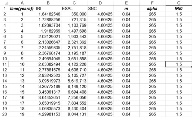
1. Presume you have obtained the following coefficients: α = 265, m = 0.04, IRI₀ = 1.5. Consider a structural number of 4.60425, ESALS on year 0 of 350,000 and growth of 3%. Estimate the amount of deterioration across time for 20 years. Use the following functional form:

$I R I_{t} = e^{m t} [I R I_{0} + a {(1 + S N)}^{- 5} N E S A L_{t}]$

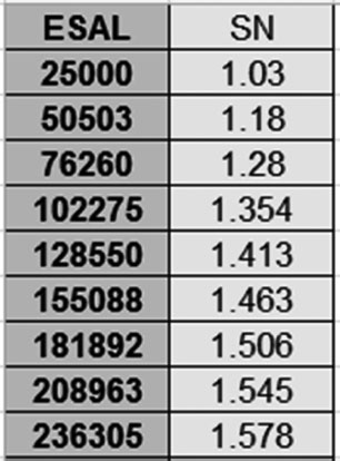
2. Estimate a coefficient to calibrate the following equation to the data in Figure 5.7.

$\log (E S A L) = 2.717 + \log {(S N + 1)}^{α}$

FIGURE 5.7
Exercise 5.2 making estimations.

ESAL is the total amount of traffic loads during the life span of the road. SN is the structural number; this value is provided on the following table. Estimate the value of the coefficient for the power of the term SN + 1.

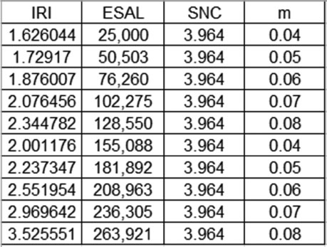
3. Estimate standardized coefficients for the environment coefficient m, the ESAL coefficient and the SNC coefficient shown in Figure 5.8. Interpret the standardized coefficients.

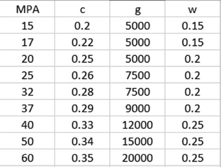
4. Use the following description to write a functional form. Add coefficients to each of the terms, and then use the data observed on the following table to estimate the value of the coefficients.

Concrete strength s depends on the amount of cement c that you add to it. It also depends on the quality of the granular aggregates g.

The other factor that we always consider is the amount of water w. If the amount of water goes beyond a certain ratio r, the strength of the mix drops. If the amount of water w drops below the minimum m, the strength of the mix drops as well. Do not use a coefficient for the water criteria. Presume m = 0.1 and r = 0.3. Figure 5.9 shows the observations that will be used for the calibration.

5. Estimate explanatory power of time, cost and comfort on utility for the data set in Table 5.5. Use STATA and the command regress.

FIGURE 5.8
Exercise 5.3 making estimations.

FIGURE 5.9
Data for Exercise 4.

TABLE 5.5
A Choice of Work Commute

Alternative	Time (Hours)	Cost ($/Month)	Comfort	Utility
1. Walk	4.5	10	3	5
2. Bike	1.18	10	4	6
3. Bus	1	101	1	5
4. Car	0.42	300	10	7
5. Walk–bus	0.82	101	0	6
6. Car–metro(1)	0.84	145	8	9
7. Car–metro(2)	1	305	9	7
8. Car–train(1)	0.92	175	7	6
9. Car–train(2)	1	175	7	5
10. Walk–train	1.25	125	6	4
11. Car–bus	0.67	151	5	5

Solutions

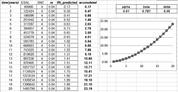
1. Figure 5.10 shows the detailed calculations associated to this specific problem.

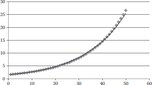
When we plot this information (Figure 5.11), we obtain a graph of IRI as the response and ESALs as the main driving factor. We can observe the speed of progression on deterioration measured through IRI.

FIGURE 5.10
Solution for Exercise 5.1 making predictions.

FIGURE 5.11
Solution for Exercise 5.1: IRI (m/Km) versus time (years).

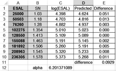
2. We will assume that the bearing capacity of the soil is 30,000. If you notice the term in the logarithm containing the ΔPSI, it goes to $\log (\frac{1}{1})$ . You can also consolidate then all constants −7.67 and 2.32 log(M_R) = 2.32 log(30, 000). The following equation shows a simplified version of the equation and will be used to estimate the value of the coefficient. We will use the least-square approach to do the estimation. Figure 5.12 shows the observed and predicted values and then uses the least-square differences to estimate the power of the coefficient. Figure 5.13 illustrates the Excel interface used for the estimation.

As seen, the value of the coefficient is 6.2.

FIGURE 5.12
Solution for Exercise 5.2 estimation of coefficient predictions.

FIGURE 5.13
Solution for Exercise 5.2 Excel interface for the estimation.

FIGURE 5.14
Solution for Exercise 5.3 estimating contribution power.

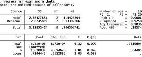
3. Figure 5.14 shows the results of the estimation using STATA. On the left side, we have the value of the coefficient and the p-value, and to the right we have the standardized coefficients. SNC is omitted because its value is fixed.

The coefficients from ESAL and m are both significant; the p-values are 0.000 and 0.025 correspondingly. The values of the coefficients are 5.51E–6 and 13.20837. If you interpret these coefficients, the contribution power of the first one goes to zero. Once you estimate the beta coefficients, you can actually see that ESALs contribute to explain more (beta = 0.75) than the environment (with a coefficient of 0.33). This means that the ESALs are $\frac{0.7519697}{0.334495} = 2.248$ times more relevant than the environment to explain the deterioration of the pavement measured through IRI.

FIGURE 5.15
Solution for Exercise 5.4 estimating α and β.

FIGURE 5.16
Solution for Exercise 5.5 simple regression.

4. The fact that we have a minimum ratio r can be linked to the amount of water on a subtraction fashion such as r − w. If the amount goes beyond r, then the value of this term becomes negative. If the amount of water does not exceed such ratio, then the value is positive. However, there is also a minimum value m so having less than m is also counterproductive. We can represent this through another ratio w − m. This means that if the amount of water drops below the minimum, this amount becomes negative as well. We can then multiply both ratios (w − m)(r − w). Figure 5.15 shows the solution.

The equation obtained before calibration is the following:

$s = c^{α} g^{β} [(w - m) (r - w)]$

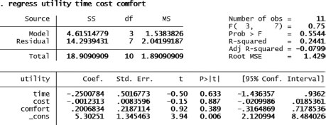
5. The simple regression of time, cost and comfort on utility result in the following coefficients and p-values. Figure 5.16 shows the solution for the coefficients, although none of these was statistically significant.

This suggests that there is no explanatory power on any of the three criteria (cost, time, comfort) to explain the level of utility.

References

1. Paterson, W. D. & Attoh-Okine, B., 1992. Simplified Models of Paved Road Deterioration Based on HDM-III. Proceedings of the annual meeting of the Transportation Research Board. Washington, DC.

2. StataCorp. 2011. Stata Statistical Software: Release 12. College Station, TX: Stata-Corp LP.