Spatial Vision
An endless shimmering expanse of tinder-dry yellow grass, broken only by an occasional grove of ancient gnarled eucalypts, bakes under the relentless Australian noonday sun. The heat, rising in great invisible shards from the ground, is palpable. Without warning, one of the world’s largest birds of prey—the wedge-tailed eagle Aguila audax—lifts slowly and deliberately from its aerie in a nearby gum tree, its huge wings climbing ladders of air to gain height. Arching leftward, it enters a vertical chimney of heat and surges heavenward in wide spirals. Atop this thermal, almost 2 km above the ground, this massive bird begins to scan the immense ochre sweep of the Monaro High Plains, a vast undulating grassland stretching westward toward Mt. Kosciuszko. The eagle is on the lookout for rabbits, now its favorite food thanks to their introduction by European settlers 200 years earlier. Its eyes, though evolved for other quarry, have astonishing visual acuity, in fact one of the best in the animal kingdom. Although at this altitude the wedge-tailed eagle is an indiscernible speck in the sky for rabbits on the ground, they themselves, and their telltale scurrying through the grass, are seen with brilliant clarity, allowing the eagle to select its target. Even though the eagle’s descent is long, the rabbit stands little chance. In fact, it seems to be oblivious to the danger descending rapidly from above. The outcome of the eagle’s stoop on its prey is almost certain.
The eagle’s visual prowess is due to a remarkable feature of the eagle’s retina. The deep dimple of the foveal surface acts as a negative lens—effectively akin to a telephoto component—that magnifies the image of the rabbit in the eagle’s retina. In contrast, the eyes of the rabbit—with their long horizontal streak of high resolution—are trained around the horizon, from where they expect land-bound predators such as foxes. With their very different eyes, eagles and rabbits underscore the major role predation has played in the evolution of spatial vision for both predator and prey alike. The same can be said for the detection and pursuit of mates. In fact, every aspect of animal life has profoundly affected the way spatial vision has evolved. Exactly how is the topic of the present chapter.
We humans are accustomed to seeing the world in high resolution—in fact, this is arguably our best-developed visual capacity. Compared to many other animals, our eyes are not particularly sensitive to light; nor is our sense of color especially good. The undoubted splendors of nature’s ultraviolet colors are totally invisible to us, as are the world’s rich natural sources of polarized light. But when it comes to discerning fine spatial detail, few animals come close to us. There are other primates that share our spatial abilities (e.g., macaques: see De Valois et al., 1974), but only some groups of birds—notably large birds of prey—significantly exceed them. In the case of wedge-tailed eagles, their large eyes, tightly packed photoreceptors, and the telephoto optics mentioned above endow them with a visual acuity that in bright light is two to three times higher than our own (Reymond, 1985). But such birds are among the exceptions.
What then do we make of the great majority of animals whose spatial resolution is considerably lower than ours—such as the dragonfly, whose two apposition compound eyes sample almost 360° of visual space with just 60,000 ommatidia? Do these few “visual pixels”—about two orders of magnitude fewer than our own—reduce the world of dragonflies to an incomprehensible blur? Anyone who has taken the time to watch dragonflies hunting and defending their territories around the edges of a sunny pond will know that the answer to this question is clearly “no.” Dragonflies have astounding spatial vision. Not only can they can pluck a fly from the air following a precise high-speed aerial pursuit (Olberg, 2012; see chapter 10), they can actively home in on a single fly in a swarm without being distracted by the movements of others, revealing a selective attention mechanism akin to that in mammals (Wiederman and O’Carroll, 2013). And as we see in chapter 11, there are many nocturnal birds and mammals with at least 10 times as many “visual pixels” as the dragonfly that have forsaken vision almost entirely and instead rely on olfaction and mechanoreception for the tasks of daily life. Thus, the sheer number of visual sampling stations possessed by the retina of an eye is a poor indicator of the ability of animals to discern and react to spatial details in a scene.
Then of course there is the nature of the spatial task that has to be solved. Some animals need to discern the arrangement of objects in an extended scene. Others need to see and localize a tiny point of light against a dark background (like a deep-sea fish viewing a bioluminescent flash) or to detect a tiny dark silhouette against a bright background (like a dragonfly chasing a fly). Some animals of course need to do both. And just as we saw earlier in chapter 4, to maximize sensitivity, eyes adapted for viewing extended scenes must be built differently from those adapted for viewing point-source scenes. As we will see, the same can be said for the maximization of spatial resolution.
But regardless of whether the visual task is to follow a tiny target or to keep track of the physical arrangements of objects in a scene, all aspects of animal life have steered the evolution of spatial vision, particularly the distribution of an eye’s sampling stations in visual space. The pursuit and interception of mates and prey, the avoidance of predators, the negotiation of a complex three-dimensional world during locomotion, and the physical layouts of different habitats have all played critically important roles in how an eye’s sampling matrix has evolved. Exactly how these ecological forces have shaped the sampling matrices of animal eyes is the major theme of this chapter.
We restrict our discussion to the two major eye types of the animal kingdom—camera eyes and compound eyes—as these are by far the best understood in terms of the ecology of spatial vision. Moreover, except where necessary in the service of visual ecology, we do not discuss the relationship between image quality and the sampling matrix, topics we introduced in the context of eye specialization in chapters 4 and 5. For a deeper discussion of this admittedly fascinating topic, the interested reader is referred to several superb accounts, notably those of Wehner (1981), Snyder (1977), Hughes (1977), Land (1981), and Land and Nilsson (2012).
Before we discuss how the ecologies of animals have driven the evolution of their sampling matrices, we begin by describing the individual sampling stations themselves and the ways in which variations in the sampling matrix have been achieved. We start by defining the parameter of most importance for this description, namely the interreceptor angle Δφ, and we do so first in camera eyes.
The Sampling Stations of Camera Eyes
Camera eyes are possessed by vertebrates as well as by a number of invertebrates (chapter 5), for instance mollusks (e.g., gastropods and cephalopods) and arachnids (e.g., spiders and scorpions).
In chapter 4 we saw that in a camera-type eye, where the sampling stations (or “receptors”) are tightly packed (and are thus touching, or “contiguous”), the interreceptor angle (Δφ) can be described by the following expression (equation 4.3b; figure 6.1A):
where d is the diameter of the receptor (μm) and f is the focal length of the eye (μm). Larger camera eyes with longer focal lengths will tend to have smaller values of Δφ and thus higher spatial resolution (incidentally, they will also tend to have larger pupils and higher sensitivity and thus better vision overall). Even in eyes of constant focal length, areas of the retina with smaller receptors will also have smaller values of Δφ and higher resolution. In this latter case such a local area of high resolution is referred to as an “area centralis” (vertebrates) or an “acute zone” (invertebrates). If in addition the retinal surface within the area centralis is inwardly dimpled to create a pit, the area is referred to as a “fovea.” Foveae result from a local absence of blood vessels and a thinning of the retinal layers overlying the photoreceptors—this thinning reduces the scattering of the incoming light that passes through these layers prior to its absorption. Simian primates (like ourselves) possess a fovea, although the pit is rather shallow. In other species foveae are often deeply pitted. These deep foveae, called “convexiclivate” by Walls (1942), occur in a wide variety of vertebrate eyes, including those of birds of prey, swallows and kingfishers, chameleons, pipefish, seahorses, and in many species of deep-sea fish. An analogous structure is also found in the retinas of jumping spiders. As we will soon see, deep convexiclivate foveae have a special role to play in spatial vision.
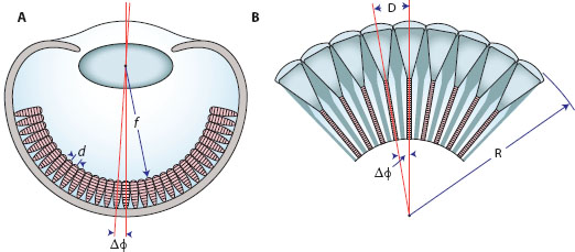
Figure 6.1 Definition of the interreceptor angle Δφ in camera eyes (A, assuming contiguous photoreceptors) and the interommatidial angle Δφ in compound eyes (B). d = interreceptor distance (equal to the receptor diameter in a contiguous retina), f = focal length of the eye, D = distance between the centers of two adjacent corneal facet lenses (equal to the facet diameter), and R = local radius of the eye surface. (Schematic drawings of the two eyes courtesy of Dan-Eric Nilsson)
In vertebrate camera eyes the tightly packed primary photoreceptors (i.e., the rods and cones; chapter 3) represent the first matrix of sampling stations that receive the focused image. In the eyes of diurnal primates such as ourselves, the cones are smallest, densest, and thus most numerous at the exact center of the fovea (figure 6.2). In the central fovea of our own eye, for instance, the cone outer segment diameter d is around 2.5 μm. Because the focal length f of the human eye is 16.7 mm (= 16,700 μm), equation 6.1 reveals that the interreceptor angle Δφ is 1.50 × 10⁻⁴ radians, or 0.009° (1 radian = 180°/π = 57.3°). This is an extremely small value—it is little wonder that our foveal vision is so acute! In fact this value of Δφ is similar in size to the smallest detail we can discriminate in bright light (when our pupil is about 2 mm in diameter), implying that our spatial vision is limited only by diffraction. In the language of spatial frequencies (see chapter 4), this means that the finest pattern of black-and-white stripes that our photoreceptor matrix can reconstruct (with Δφ = 0.009°) has a spatial frequency of around 60 cycles/°. This turns out to be roughly the same value as our optical cutoff frequency at the diffraction limit in green light (see figure 4.9).
Diffraction-limited optics matched to the sampling matrix is also a feature of other anthropoid primates as well as large birds of prey. However, in other vertebrates image quality can be much poorer than implied by the photoreceptor sampling matrix. For instance, the small (6-mm-diameter) rod-dominated eyes of the nocturnal brown rat Rattus norvegicus have Δφ = 0.025° (foveal rods). When rat eyes are fully dark-adapted (pupil diameter around 2.5 mm), the smallest spatial detail resolvable in the optical image is 0.41° wide—16 times wider than Δφ (Clarke and Ikeda, 1985; Hughes and Wässle, 1979)! Even in bright light, when the pupil is eight times narrower, the smallest resolvable detail is only a third smaller. This means that the matrix of rods is able to reconstruct much finer spatial details than the optics can supply, indicating that either aberrations and other optical imperfections (rather than diffraction) limit the performance of the eye or that a coarser matrix of under lying ganglion cells provides the limit. As we discuss below, the ganglion cells usually pool signals from large groups of photoreceptors, especially in the retinal periphery, but in nocturnal animals such as the rat this can occur even in the fovea, where it increases sensitivity (see chapter 11). Indeed, Δφ for the foveal matrix of ganglion cells is about 0.16° (Hughes, 1977), six times the value for the rod matrix. However, this is still less than half the size of the smallest spatial detail resolvable in the optical image. Thus, the bottleneck for spatial vision is the optics, a conclusion that in fact manifests itself in the rat’s behavior—the smallest spatial detail it can discern in dim light is around 0.4° in size (Birch and Jacobs, 1979; see figure 11.4), very close to the smallest passed by the optics. Interestingly, even in our own eyes, when the pupil is wider than about 3 mm (at moderate light levels), image quality also worsens due to spherical and chromatic aberration, with a corresponding loss in acuity (Charman, 1991).
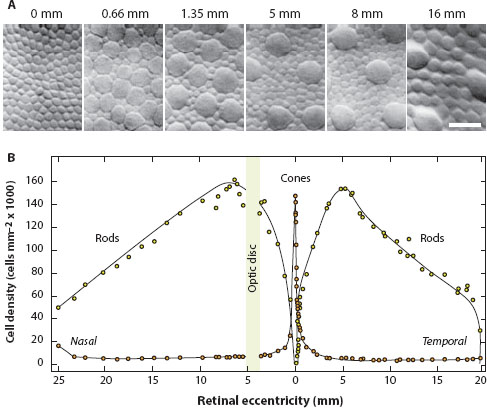
Figure 6.2 Densities of rods and cones in the human retina as a function of distance (eccentricity in millimeters) from the fovea (eccentricity = 0 mm). (A) Transverse sections through the mosaic of photoreceptor inner segments at different eccentricities. The center of the fovea (0 mm) is free of rods, and the cone inner segments (seen here) are extremely narrow. At an eccentricity of 0.66 mm (moving temporally), the cone inner segments have become much wider and less densely packed (large profiles), and this trend increases with increasing eccentricity. Rod inner segments (small profiles), narrow and relatively few at 0.66 mm, increase in number and prominence with increasing eccentricity. Scale bar = 10 μm. (Compiled from images in Curcio et al., 1990, and reproduced with permission of the publisher, John Wiley & Sons) (B) The relative densities of rods and cones along a nasal-temporal transect passing through the fovea (0 mm). Notice how rods and cones change their relative dominance at different locations in the retina. (Adapted from Rodieck, 1998, from data originally published by Østerberg, 1935).
But let us again return to the human retina. As one moves away from the foveal center, the cone size increases rapidly, and their density falls (figures 6.2A and 6.3C), plateauing to a steady low density throughout the remainder of the retina. At a distance of 8 mm (i.e., at an “eccentricity” of 8 mm) from the foveal center, d has increased from 2.5 μm to around 19 μm (figure 6.2A: because the cones are not contiguous, d is the distance between cone centers). Thus, Δφ becomes correspondingly larger, around 0.065°, or over seven times larger than in the central fovea.
Interestingly, the density profile for rods is completely different (figure 6.2B). The rods instead are totally absent from the foveal center but quickly rise in number and density to become most numerous at some distance away from the center (in humans around 5–7 mm away). Beyond this peak, rod density declines slowly throughout the remainder of the retina. As we see in chapter 11, this distribution of rods and cones is radically different in the eyes of nocturnal primates such as the owl monkey Aotus, and (as we will also see below) for good reason. But regardless of species, the interreceptor angles (Δφ) for rods and cones in vertebrate eyes will vary markedly from one part of the retina to another. Moreover, because the fovea is cone dominated and the peripheral retina is rod dominated, this variation in Δφ will also differ for the two photoreceptor types.
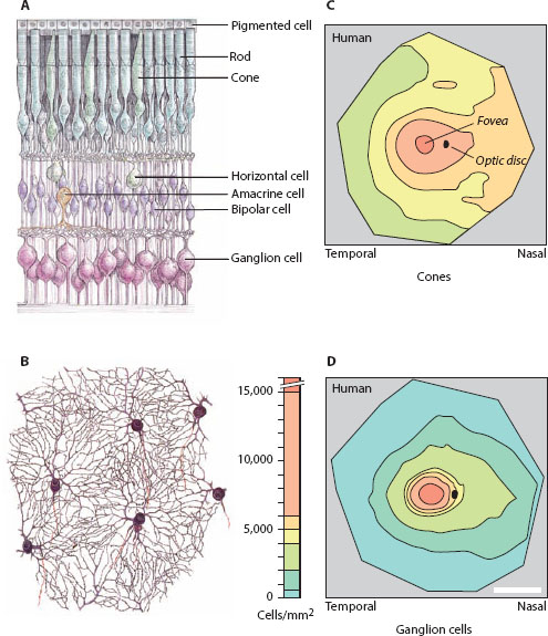
However, despite their large variations, the matrices of rods and cones do not define the visual sampling stations of the vertebrate retina. Instead, the sampling stations are defined by the retinal ganglion cells, the cells to which the photoreceptors ultimately converge (figure 6.3A; Hughes, 1977; Rodieck, 1998; Collin, 1999; Peichl, 2005). In mammals each cone is connected to two kinds of cone bipolar cells—an ON cone bipolar cell and an OFF cone bipolar cell. These in turn respectively connect to two kinds of ganglion cells—an ON ganglion cell and an OFF ganglion cell. As their names suggest, the ON cells create an ON pathway (which is activated by an increase in illumination), whereas the OFF cells create an OFF pathway (which is activated by a decrease in illumination). The rods also connect to bipolar cells, specifically to rod bipolar cells (which are all of the ON type). These each connect to an amacrine cell (see figure 6.3A), the so-called AII amacrine cell, which in turn connects to one ON and one OFF cone bipolar cell. As before, these connect respectively to one ON ganglion cell and one OFF ganglion cell. Thus, in a sense, the rods converge onto ganglion cells by piggybacking onto the cone circuitry.
But irrespective of the specific circuitry that underlies the convergence of rods and cones onto the underlying ganglion cells, and irrespective of the complicating fact that the ganglion cells effectively form two parallel matrices (an ON matrix and an OFF matrix), a critically important principle remains: each ganglion cell receives input from one or more photoreceptors, the exact number depending intimately on the eccentricity where the ganglion cell is located. At the very center of the fovea, one single “midget” ganglion cell receives input from one single cone. As its name suggests, the receptive field of a midget ganglion cell—which is defined by the extent of its dendritic field—is very small. In fact, it is no larger than the receptive field of the cone itself. But as soon as one moves away from the foveal center, the number of photo receptors supplying single ganglion cells grows. Within a couple of millimeters of the foveal center many tens of cones are supplying each ganglion cell (with a dendritic field that has expanded appropriately). In the retinal periphery, which is dominated by rods, thousands of rods may converge onto single ganglion cells. Not surprisingly, the dendritic fields of peripheral ganglion cells (especially those of the “parasol” type) are enormous.
Because the dendritic fields of the ganglion cells tend to “tile” the retina in a regular mosaic with little overlap (Rodieck, 1998; figure 6.3B), an increase in the size of the dendritic (receptive) field implies a decrease in ganglion cell density (figure 6.3D). Thus, at any one location in the retina, the dendritic field size of the ganglion cells (now determining d in equation 6.1) defines the local Δφ: the smaller the dendritic fields of the ganglion cells (and the higher their density), the smaller the value of Δφ and the higher the local spatial resolution. Ganglion cell dendritic fields—and values of Δφ—are thus smallest in the fovea. As one moves away from the fovea, the dendritic fields of the ganglion cells gradually become larger (with a concomitant increase in Δφ), and the local spatial resolution falls.
Figure 6.3 Retinal ganglion cells, the sampling stations of the vertebrate retina. (A) Main cell types of the vertebrate retina, showing the retinal ganglion cells that send information processed by the retina to the brain for further processing. In this drawing, light enters the retina from below. (From Hubel, 1995, with permission from Macmillan Publishers Ltd.) (B) A drawing of a network of parasol ganglion cells from the human retina, showing their packing arrangement. (From Rodieck, 1998, using data originally published by Dogiel, 1891, with permission from Sinauer Associates) (C,D) The spatial density of cones (C) and all classes of ganglion cells (D) in a flat-mounted human retina (color scale in D applies to both panels). In the fovea the density of the two cell types is similar, and at its very center there is a 1:2 convergence of cones onto (midget) ganglion cells (see text). However, at increasing eccentricity, the density of ganglion cells falls much more quickly than that of cones, implying that ever-larger pools of cones converge onto single ganglion cells. Scale bar = 10 mm. (Adapted from Rodieck, 1998, from data originally published by Curcio et al., 1990)
Take the midget ganglion cells as an example. In the human retina these constitute 70% of all ganglion cells and are found throughout the retina—most of the remaining 30% is comprised of “parasol” ganglion cells (with larger dendritic fields), bistratified ganglion cells, and photosensitive ganglion cells involved in the control of the circadian rhythm. As mentioned above, midget ganglion cells have their smallest receptive fields at the center of the fovea, where they collect inputs from single cones. Thus, as for the cones, the interreceptor angle Δφ for human foveal midget ganglion cells will be 0.009°. However, at an eccentricity of 8 mm, where Δφ for the cones is 0.065° (see above), midget ganglion cell dendritic fields are about 90 μm across (Dacey, 1993). This results in Δφ = 0.31°, a value nearly five times greater than the value for cones. At the same eccentricity, Δφ for the parallel matrix of parasol ganglion cells would be more than three times larger again. Not surprisingly, density plots for cones and ganglion cells (of all types) across the human retina reveal similar high densities near the fovea, but everywhere else the density of the ganglion cells (i.e., the density of the retina’s sampling stations) is much lower than that of the cones (compare figures 6.3C and D).
Invertebrate Camera Eyes
In invertebrate camera eyes the situation is a lot simpler thanks to the existence of only one visual cell type in the retina, the photoreceptor. In this case spatial vision could potentially be subserved by the full density of the photoreceptor matrix (and not by an underlying and more dilute matrix of other cells such as the ganglion cells we discussed above).
In squid and octopus—whose camera eyes can be quite massive (see figure 11.6)—the spatial resolution could potentially be extremely high. In the enormous eyes of the giant deep-sea squid Architeuthis dux (which can reach around 30 cm in diameter; see chapter 11), the rhabdom diameter d is around 4 μm, and the focal length f of the eye is around 110,000 μm (see table 4.1). The interreceptor angle Δφ is then about 0.002° (equation 6.1), almost five times smaller than the smallest foveal value in our own eye (and probably the smallest value in the animal kingdom). Whether this deep-sea creature, which inhabits the inky depths about 1 km below the surface of the sea, actually achieves this resolution is hard to say—the optical quality of the image might be much worse than that needed to match the full resolution of the retina (due to aberrations and other optical problems), as we saw above for rats. Even more likely is that the photoreceptors are summed together into groups to increase sensitivity, a strategy that compromises spatial resolution (by effectively widening Δφ). In smaller cephalopods (with smaller eyes) living in bright light (such as Octopus) image quality could be better and summation unnecessary, in which case a much higher resolution might be attained. Nevertheless, in Octopus vulgaris (whose eyes are 10–20 mm across and where Δφ is around 0.02°) the smallest detail that can be discriminated behaviorally is about five times larger than Δφ (Muntz and Gwyther, 1988), implying that lens aberrations could indeed be a limitation to resolution in cephalopods.
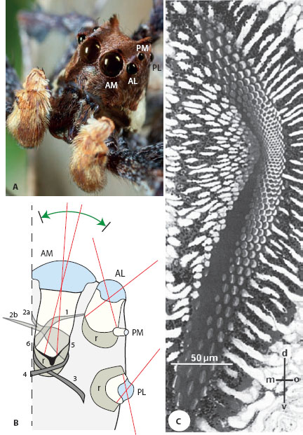
Figure 6.4 The eyes of jumping spiders. (A) A portrait of the male jumping spider Portia fimbriata, which has the highest acuity known in spiders. One eye of each of the four pairs of eyes is labeled. AM = anteromedial eyes, AL = anterolateral eyes, PM = posteromedial eyes, PL = posterolateral eyes. (Image reproduced with the kind permission of Jürgen Otto) (B) A schematic transverse section through the right-side head and eyes of a jumping spider showing the visual fields of each eye (red lines). The long tubular AM eyes are the largest and have a retina (r) at the base consisting of four layers (I–IV). Six muscles (1–6) scan each AM eye tube over a wide arc (horizontal extent is shown by green arrow), and thus compensate their narrow visual fields (5° horizontally by 20° vertically). (After Land and Nilsson, 2012) (C) A transverse light microscope section through retinal layer I in an AM eye of the jumping spider Phidippus johnsoni showing its elongated dorsoventral shape. Notice how the density of photoreceptors (and thus the spatial resolution) increases dramatically toward the center of the retina. d = dorsal, v = ventral, m = medial, o = outer. (From Blest et al., 1988)
The same conclusion can be drawn for the camera eyes of most web-building spiders, whose eyes are usually poorly resolved, and which instead rely on mechanosensory cues to catch prey. Nonetheless, some spiders (e.g., the nocturnal wolf spiders and net-casting spiders or the day-active jumping spiders Salticidae) hunt visually. Of these, the jumping spiders have stunningly well-resolved eyes. The fringed jumping spider Portia fimbriata, a native of Southeast Asia and Australia, is an excellent example. Like most spiders, Portia has eight eyes arranged around the front, sides, and top of the head carapace (figure 6.4A): two anterolateral (AL) eyes, two posterolateral (PL) eyes, two posteromedian (PM) eyes, and two anteromedial (AM) eyes. The first three pairs are collectively referred to as the “secondary eyes,” whereas the AM eyes—which in jumping spiders are overwhelmingly the largest—are referred to as the “principal eyes.” The AM eyes are also the most acute—their tubular form houses a long focal length, a sharp lens, and the presence of a deep image-magnifying convexiclivate fovea (see figure 6.5A), all of which ensure a crisp image. The fovea itself has tightly packed photoreceptors (figure 6.4C), which in Portia are separated by an astonishingly small interreceptor angle of just 0.04°, the smallest value known in any spider and quite possibly in any arthropod. This is only five times coarser than in our own fovea, but in an eye thousands of times smaller!
As we will also see for the tubular eyes of owls and deep-sea fish (chapter 11), the downside of the tubular shape and high resolution of the AM eyes is that they have a restricted field of view (figure 6.4B): in the jumping spider Phidippus johnsoni (Land, 1985) this is only 5° horizontally and 20° vertically (compared to 135° in their nontubular PL eyes). To compensate for this, six muscles in two bands scan the ocular tube behind the stationary lens, allowing spiders to scan prey and conspecifics and to build up a high-resolution image over time (see chapter 10). The secondary eyes, in contrast, with their lower resolution and broader fields of view, are specialized for alerting the spiders to movements at the side. Once registered, these movements lead to a rapid jump of the spider to face (and then scan) the object of interest with the AM eyes.
Negative Lenses and Telephoto Components
Both jumping spiders and birds of prey such as the Australian wedge-tailed eagle extend their spatial resolution even beyond that of their already tightly packed sampling stations by taking advantage of the deeply curved inner surface of their foveal pits (figure 6.5A,B). Because the retinal tissue has a slightly higher refractive index than the vitreous (1.369 vs. 1.336), the foveal surface acts as a negative (diverging) lens, which effectively lengthens the focal length of the eye and magnifies the image within the fovea, very much like a telephoto lens in a camera (figure 6.5C). In the small heads of jumping spiders this is particularly useful as it effectively mimics a longer and better resolved eye but in a smaller format (albeit at the cost of a reduced visual field). In Portia, the powerful foveal lens magnifies the image by over one and a half times, increasing the finest spatial frequency that the matrix of layer 1 photoreceptors can reconstruct from around 7.8 cycles/° (without the foveal pit) to 12.4 cycles/° (Williams and McIntyre, 1980).
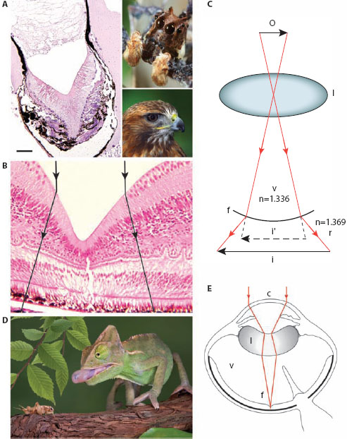
Figure 6.5 Negative lenses in camera eyes. (A,B) Foveal pits in the retinas of the tubular AM eye of the jumping spider Portia fimbriata (A with inset) and the red-tailed hawk Buteo jamaicensis (B with inset). Scale bar in A = 50 μm. Ray paths for the foveal negative lens in B are shown in black. (Photo credits: Jürgen Otto and Nialat: 123RF.com photo agency. Histological sections by Richard Dubielzig DVM courtesy of Ivan Schwab, from Schwab, 2011, with permission from Oxford University Press) (C) Enlargement of an image by the diverging back element of a telephoto system (in this case foveal pit f, which separates the vitreous v [of lower refractive index n] from the retina r [of higher n]). By virtue of the foveal back element, the lens focuses an image i of an object o that is magnified relative to the image (i′) that would have been formed had the element not existed. (Adapted from Williams and McIntyre, 1980, with values of n from Land and Nilsson, 2012) (D) The veiled chameleon Chamaeleo calyptratus. (Photo credit: Cathy Keifer: 123RF.com photo agency) (E) Image formation in the eye of Parson’s chameleon, Calumma parsonii. The cornea c acts as a positive (converging) lens, and the curiously shaped internal lens acts as a negative (diverging) lens. Together the cornea and lens act as a Galilean telescope, effectively increasing the focal length of the eye and magnifying the image. A deep convexiclivate fovea magnifies the image even further. Other abbreviations as in C. (Image adapted from artwork by Tim Hengst with permission from Ivan Schwab; from Schwab, 2011, with permission from Oxford University Press)
Similar conclusions can also be drawn for birds of prey. The foveal pit of the hawk (figure 6.5B) also magnifies the image by about one and a half times (Snyder and Miller, 1978), and with the same benefits. Despite having eyes about the same size as our own, the finest spatial frequency hawks can discriminate behaviorally is around 140 cycles/° (Reymond, 1985), more than twice our upper limit (60 cycles/°). Even though this gain is mostly due to the diverging foveal pit, the hawk’s denser packing of foveal photoreceptors and three-times-wider daytime pupil (which improves the diffraction limit) also contribute.
An even stranger negative lens can be found in the curious eyes of chameleons (figure 6.5D,E). Chameleons are well known for their completely decoupled turret-like eyes that independently scan different regions of space in search of insect prey, only recoupling for a final frontal attack, which involves a lightening-fast and well-aimed firing of their sticky tongue (figure 6.5D). Each eye is also capable of a fast and powerful accommodation that allows precise monocular depth perception for accurate estimation of prey distance (Ott and Schaeffel, 1995), an ability that relies on the accurate focusing of a magnified image. This magnification is achieved by the oddly shaped internal lens which, unlike in every other vertebrate eye known, is negative rather than positive (figure 6.5E). In combination with the strongly positive cornea, this negative lens increases the focal length of the overall optical system (much as a camera’s telephoto lens does) and thus magnifies the image. The image is magnified even further by the chameleon’s deep convexiclivate fovea.
The Sampling Stations of Compound Eyes
The interreceptor angle Δφ of a compound eye is simply defined by the density of ommatidia (per unit visual angle). This is nicely illustrated by considering two extreme examples: large aeshnid dragonflies, which may possess as many as 30,000 ommatidia in each of its apposition eyes, and some groups of primitive ants that may possess fewer than 10. If the eyes of both insects view the same solid angular region of visual space, then the dragonfly will sample that region with vastly greater spatial resolution, simply because of its much higher density of sampling stations (i.e., ommatidia). This density is directly related to the local “interommatidial angle” Δφ (figure 6.1B): smaller values of Δφ indicate a greater sampling density and a higher spatial resolution. The interommatidial angle depends primarily on two anatomical parameters, the facet diameter, D and the eye radius, R:

A larger local eye radius (i.e., a flatter eye surface) or a smaller facet produces a smaller interommatidial angle. However, there is a limit to how much Δφ can be narrowed by decreasing the size of the facet because, as we saw in chapter 4, the size of the Airy disk (λ/D radians, where λ is the wavelength of light) will become unacceptably large if D becomes too small. Nevertheless, it is possible to have a region of the eye with such a large radius of curvature that an extremely small Δφ is still possible without having to sacrifice facet size. In fact in many apposition eyes the facets in these regions can actually be much larger than in other regions of the eye with double the Δφ (which is better for both diffraction and sensitivity)! This can readily be seen, for example, in the fly Syritta (Collett and Land, 1975), where in the flattest region of the eye (with R = 3.8 mm) the facets are at their maximum size (D = 40 μm). Here Δφ is just 0.6° (equation 6.2). In another region of the eye, where the facets are less than half the size (D = 18 μm), Δφ is two and a half times wider (1.5°). This is simply because the eye surface here is highly curved, having an eye radius over five times smaller (R = 0.7 mm). The flattened frontal eyes of a long-legged fly (figure 6.6B), which have massive facets and very narrow Δφ, provide another good example.
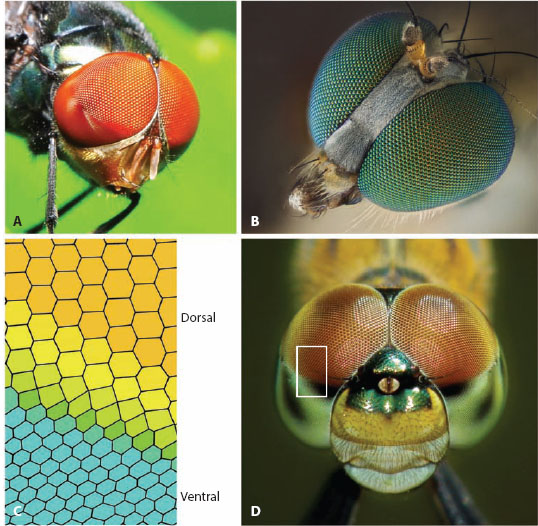
Figure 6.6 Acute zones and bright zones in apposition compound eyes. (A) The blowfly Chrysomyia megacephala (male) showing the sudden enlargement of corneal facets in the dorsal part of the eye that indicates the presence of a bright zone (used for detecting and intercepting females). (B) The head of a long-legged fly (Family Dolichopodidae) with huge anterior corneal facet lenses that indicate the presence of a frontal acute zone (used in prey capture). (Photo credit: Laurie Knight: www.laurieknight.net) (C,D) Unknown species of dragonfly (D) with a distinct dorsal acute zone of enlarged corneal facet lenses—note the sudden transition to these larger facets from the ventral to the dorsal halves of the eye (which is also accompanied by a sudden change in corneal pigmentation). This transition (indicated by the white box in D) is shown schematically in C. (Photo credit: Nattapol Sritongcom: 123RF.com photo agency. C adapted from Trujillo-Cenoz, 1972)
Thus, particularly in apposition eyes, facet diameter and eye radius can both vary dramatically within a single eye, which means that the local interommatidial angle can also vary dramatically—some directions of visual space can thereby be sampled much more densely than others. Such high-resolution “acute zones” (Horridge, 1978) are common among insects and crustaceans and, just as with the functionally equivalent foveae of vertebrates, the placement and size of an acute zone reflect the habitat and ecological needs of the eye’s owner. The dramatic increase in facet size in the dorsal eye regions of many dragonflies (figure 6.6C,D) is an excellent example. As we see below, this distinctive region, which is easily visible to the naked eye, is an acute zone specialized for the detection of prey.
Interestingly, however, an eye region of large facets does not always signal the presence of an acute zone. In the males of a couple of notable species of flies—the blowfly Chrysomyia megalocephala (figure 6.6A) (Hateren et al., 1989) and the hoverfly (dronefly) Eristalis tenax (Straw et al., 2006)—the dorsal eye regions have enlarged facets but maintain large interommatidial angles and wide rhabdoms. In other words the enlarged facets are not associated with increased resolution, as in an acute zone, but with increased sensitivity. These regions have thus been aptly named “bright zones.” Because they have so far been found only in males, bright zones are probably used primarily for the detection and pursuit of mates. The chief advantage of a bright zone is that it supplies more photons and increases the visual signal-to-noise ratio and thus the contrast sensitivity. For the detection of a small moving target this strategy could be quite useful, especially in dimmer light. Indeed, the dronefly’s bright zone enhances the speed and contrast sensitivity of responses from motion-sensitive cells in its lobula, improvements beneficial for both the detection of small moving targets and the control of hovering.
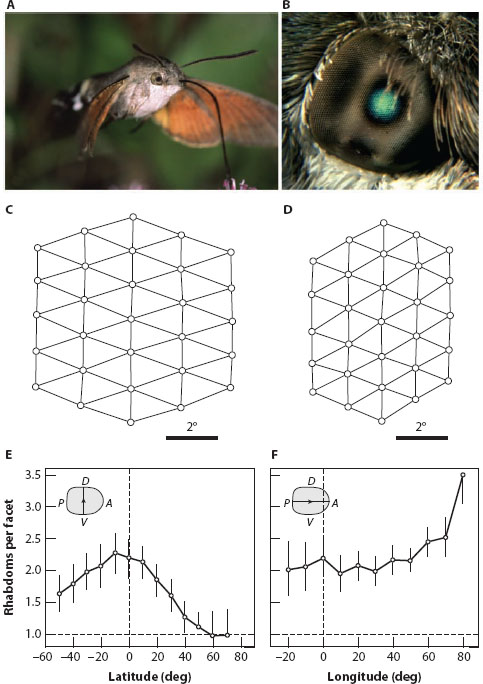
Although common in apposition eyes, the spherical shape (i.e., constant eye radius) and strict optical design of superposition eyes exclude the creation of acute zones. One remarkable exception does, however, exist: the highly nonspherical refracting superposition eyes of the hummingbird hawkmoth Macroglossum stellatarum (figure 6.7A). Somehow during development the facet lenses and rhabdoms have become decoupled to produce many more rhabdoms than facets. The rhabdoms have then been arranged to form local acute zones, their local angular packing (figure 6.7C,D) bearing no resemblance to that of facets in the overlying cornea. There are two acute zones, one frontal and slightly ventral, where there are up to four rhabdoms per facet, (figure 6.7F) and another providing improved resolution along the equator of the eye, with over two rhabdoms per facet (figure 6.7E). Moreover, the size of the facets and the area of the superposition aperture (figure 6.7B) are both maximum over the frontal retinal acute zone. By having larger facets, a wider aperture, and denser rhabdom packing, Macroglossum’s frontal acute zone provides the eye with its sharpest and brightest image and samples it with the densest photoreceptor matrix. It is this eye region that Macroglossum uses to fixate flower entrances during hovering and feeding and is no doubt one of the most important parts of its eye. How the eye pulls off this optical feat is still unknown, but it clearly provides better visual performance—at least in the frontal visual field—than a conventional superposition eye of the same size (Warrant et al., 1999).
Figure 6.7 An acute zone in the retina of a superposition compound eye. (A) The hummingbird hawkmoth Macroglossum stellatarum. (B) Unlike in a classical superposition eye, the moth’s super position aperture (equivalent to its greenish eye glow) varies in size and is largest in the frontal eye, the region used for stabilizing the flower entrance while hovering during feeding. (Images courtesy of Michael Pfaff) (C,D) The retinal sampling matrix of rhabdoms is coarser in the lateral (C) than in the frontal (D) part of the eye. The small circles represent the rhabdom centers. (E,F) The number of rhabdoms per facet along the dorsoventral meridian (longitude 0°; E) and along the posterior-anterior equator (latitude 0°; F). D = dorsal, V = ventral, A = anterior, P = posterior. (Panels C and D from Warrant et al., 1999)
Despite their great benefits, foveae and acute zones rarely view more than a small fraction of the eye’s visual field. The reason for this lies in an unavoidable visual constraint—its energetic cost. The energy required per unit solid angle of visual space is much higher in an acute zone or fovea simply because the density of energy-craving photoreceptors—not to mention the cost of additional processing power required in the central nervous system—is much greater than in other parts of the eye. And as shown in flies (see below), acute-zone photoreceptors can be faster, sharper, and code more information than those in other eye regions, which elevates the energetic cost even further (Burton et al., 2001). Not surprisingly, the longer eye radius—a proxy for a larger eye—and the extra energetic expense are simply unsustainable in more than just a small region of the eye. Thus, the presence of a fovea or acute zone invariably implies that the region of the world being so finely and expensively sampled is of utmost ecological importance.
What then might be so important? It turns out that many aspects of animal life have manifested themselves in the layout of the eye’s sampling stations and in the extent and location of foveae and acute zones. The urge to find a partner, the endless search for food, and the vigilant watchfulness required to spot predators and avoid being devoured are three such aspects. A fourth is the physical layout of the habitats where animals live because this determines the probabilities with which relevant objects can be seen in different directions. A fifth aspect, and the one we discuss first, is “optic flow”—the way the spatial details of the world flow past an animal as it moves through its environment. All these aspects of animal life have invariably led to the evolution of sensory “matched filters,” a concept first introduced by Rüdiger Wehner in 1987, whereby the spatial layout of the photoreceptor matrix is matched to the spatial demands of the specific task to be solved. Of course to perceive “the world through such a matched filter,” to quote Wehner himself, “severely limits the amount of information the brain can pick up from the outside world, but it frees the brain from the need to perform more intricate computations to extract the information finally needed for fulfilling a particular task” (Wehner, 1987). Nowhere is this truer than in the ecology of spatial vision.
Locomotion and Optic Flow
Flying insects such as butterflies, flies, bees, grasshoppers, and dragonflies have equatorial gradients of spatial resolution that are adaptations for forward flight through a textured environment (Land, 1989a). As we discuss further in chapter 10, when an insect (or any animal) moves forward through its surroundings, its eyes experience an optic flow of moving features (Gibson, 1950; Wehner, 1981). Features directly ahead appear to be almost stationary, whereas features to the side of this forward “pole” appear to move with a velocity that becomes maximal when they are located at the side of the eye, 90° from the pole. If the photoreceptors sample photons during a fixed integration time Δt, the motion of flow field images from front to back across the eye will cause blurring. An object moving past the side of the eye (with velocity v°/s) will appear as a horizontal spatial smear whose angular size will be approximately vΔt°. This effectively widens the local optical acceptance angle (Δρ, see chapter 4) to a new value of {Δρ2 + (vΔt)2} (Srinivasan and Bernard, 1975). The extent of this widening is worse at the side of eye (higher v) than at the front (lower v). In order to maintain an optimum sampling ratio of Δρ/Δφ (Snyder, 1977), the equatorial increase in Δρ posteriorly should be matched by an increase in Δφ. This indeed seems to be the case in many flying insects. For instance, in the Empress Leilia butterfly Asterocampa leilia, Δφ increases smoothly along the equator from the front of the eye to the side, from 0.9° to 2.0° in males and from 1.3° to 2.2° in females (Rutowski and Warrant, 2002).
An accurate real-time analysis of optic flow is critical for the control of flight and is the major task of wide-field motion-detecting neurons in the lobula and lobula plate regions of the insect’s optic lobe. We return to this topic in chapter 10.
Sex
The urgency to reproduce has led to some of the most spectacular visual adaptations found in nature, specifically among the invertebrates and particularly in males. This sexual dimorphism can reach remarkable proportions in the external designs of male eyes. Even the underlying visual circuitry has not escaped: in males there are entire pathways of finely tuned neurons that ascend from the eyes to steer sexual behavior.
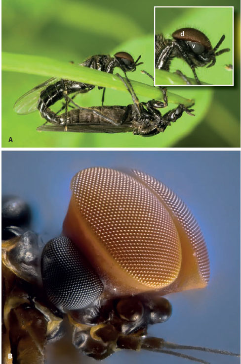
Visual sexual dimorphism, if it exists at all, is curiously hidden in vertebrates. But in insects it is often glaringly obvious (figure 6.8), with males sometimes possessing entirely separate eyes exclusively devoted to sex. In march flies and mayflies, for instance, the eye has become bilobed, with the upper lobe heavily flattened to drastically increase the retinal sampling density within a narrow upward field of view (Zeil, 1983a). It is here, silhouetted against the brighter sky, that females and rivals will appear as small dark moving spots (Zeil, 1983b). In some species of mayflies each male eye is divided into a huge dorsal “turbanate” superposition eye and a smaller ventral apposition eye. Because mayflies typically swarm at dusk and dawn, the male’s superposition eyes likely provide the extra light catch and greater contrast sensitivity needed for spotting small dark females against the backdrop of a dim crepuscular sky.
It is easy to see why good contrast sensitivity (rather than high spatial resolution per se) is important for detecting small dark targets: the ability of a photoreceptor to detect a tiny dark spot passing through its receptive field is actually limited by the smallest amount of dimming that it can just discriminate against the background. It turns out that this smallest amount of dimming can occur when the angular size of the spot is much smaller than the photoreceptor’s acceptance angle Δρ—the drone honeybee Apis mellifera (Δρ = 1.28°), with huge dorsal acute zones, will take flight and chase a queen when she subtends as little as 0.41° at the eye. Such a target will reduce ommatidial illumination by only 8% (Vallet and Coles, 1993). This indicates that good contrast sensitivity—and not simply high spatial resolution—is critically important for detecting small moving targets.
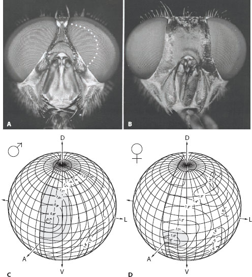
Sexual dimorphism in eye design need not be as brazen as in march flies and mayflies. In many species of brachyceran flies sexual dimorphism is subtler: the males have eyes that nearly (or completely) touch along the midline of the head, whereas in females the eyes remain widely separated (figure 6.9A,B). The extra piece of eye possessed by the male—which is amusingly referred to as a “love spot”—is used exclusively for the detection and high-speed pursuit of females (Land and Eckert, 1985). Love-spot ommatidia are distinguished by their extra-large facet lenses—depending on the species these subserve either an acute zone (as in the blowfly Calliphora and the hoverfly Volucella pellucens, figure 6.9C) or a bright zone (as in the dronefly Eristalis and the blowfly Chrysomyia, figure 6.6A). The acute zone is clearly seen in the male hoverfly Volucella, which has large love spots located frontally, 20° above the equator (figure 6.9C). The interommatidial angle Δφ here falls to just 0.7°. The size of the acute zone (the eye region where, say, Δφ < 1.1°) occupies 2230 deg2 of the visual field (shaded area in figure 6.9C). In females there is also an acute zone, but instead it is directed frontally (figure 6.9D). Δφ only falls to 0.9°, and the area of the acute zone (Δφ < 1.1°) is a mere 23% as large as that of males (510 deg2: shaded area in figure 6.9D).
Figure 6.8 Double eyes and sexual dimorphism in insects. (A) Male march fly Dilophus febrilis (Family Bibionidae) with its enormous flattened dorsal (d) apposition eyes and smaller ventral (v) apposition eyes (inset) copulates with a small-eyed female. (Image used with permission of the photographer, Dr. Ray Wilson, UK) (B) Unknown species of male mayfly showing the enormous “turbanate” dorsal superposition eyes and the smaller ventral apposition eyes. Two small bulbous eyes below the dorsal eyes are the ocelli. (Photo credit: Laurie Knight: www.laurieknight.net)
Figure 6.9 Optical sexual dimorphism in the apposition eyes of flies. (A,B) Male (A) and female (B) blowfly heads (Calliphora erythrocephala). Note how the eyes of males almost touch, whereas those of females are quite separated. The extra eye surface—or “love spot”—of males (dotted white line) provides the input to a sophisticated neural pathway for detecting and chasing females. (Images from Strausfeld, 1991, with kind permission from Springer Science+Business Media) (C,D) In the hoverfly Volucella pellucens the male love spot is a large dorsofrontal acute zone where interommatidial angles are small (C) and facet diameters are large. The visual fields of the left-eyes of the two sexes and interommatidial angles shown by isolines are projected onto spheres. Females have a much smaller frontal acute zone (compare the shaded regions, where Δφ < 1.1°). D = dorsal, V = ventral, A = anterior, L = lateral. (From Warrant, 2001)
The acute zones of male flies are not restricted to the eye surface. Below the eye there is an intricate neural pathway that is specific to males. First, the connections of photoreceptor axons to the lamina are quite different in the acute zone compared to both the female’s eye and the rest of the male’s eye (e.g., houseflies: Franceschini et al., 1981). In most ommatidia, six of the eight photoreceptors (R1–R6) are green sensitive and together synapse onto a single second-order neuron in the lamina (the first optic ganglion of the optic lobe). The remaining two (R7 and R8) are instead ultraviolet sensitive and send their axons straight through the lamina to synapse in the second optic ganglion, the medulla. Curiously, however, in the ommatidia of the male love spot, R7 mimics R1–R6, being green sensitive and (with the others) synapsing onto the same second-order lamina cell rather than continuing on to the medulla. This neural trick boosts the visual signal-to-noise ratio by 7% and thereby increases the contrast sensitivity for small moving targets.
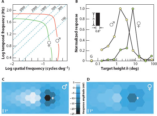
This is not the only peculiarity of love-spot photoreceptors. In houseflies they are also 60% faster than the photoreceptors of females and much more acute, with acceptance angles (Δρ) that are a little more than half those of females (Hornstein et al., 2000). This is reflected in a spatiotemporal contour plot of photoreceptor response gain as a function of spatial and temporal frequency (figure 6.10A): there is no spatial or temporal frequency where female photoreceptors outperform those of males. The diagonal lines are lines of equal angular velocity (°/s) and highlight why male love-spot photoreceptors are so much better suited to the high-speed pursuit of a rapidly turning small target such as a female fly. At the level of response shown in figure 6.10A, a spatial frequency of 0.1 cycles/° moves at 750°/s in males but at only 200°/s in females. Put in another way, a small target moving at high speed may easily be seen by males when totally invisible to females.
The reason spatial resolution is so much better in love-spot photoreceptors is that the overlying facet lenses are large (good photon catch and a narrower Airy diffraction pattern), and the rhabdomeres are unusually thin. The improved response speed is achieved by a faster transduction mechanism and a tuned voltage-activated conductance that enhances the membrane’s frequency response. In fact, in the blowfly Calliphora vicina, this translates into an information rate (in bits/s) in male photoreceptors that is up to 40% higher than that in females (Burton et al., 2001). All these photoreceptor modifications dramatically improve the visibility of a small rapidly moving target. The neural contrast of such a target—both in space and in time—is significantly enhanced in the responses of male love-spot photoreceptors compared to the responses of female photoreceptors (figure 6.10C,D). Of course, as we mentioned above, all this only comes at a cost—the extra tuned conductance (which involves the passage of ions through dedicated channels in the photoreceptor membrane) and the production of larger lenses are all energetically expensive.
Higher up in the fly’s optic lobe, the sexual dimorphism introduced in the eyes is maintained. Here, in the lobula of males, large male-specific visual cells respond maximally to small dark objects moving across the frontal-dorsal visual field corresponding to the love spots (Strausfeld, 1991; Gilbert and Strausfeld, 1991; Gronenberg and Strausfeld, 1991). Such cells are clearly suited to the detection of females (that incidentally lack this circuitry). One such group of cells—the small-field small-target movement detectors (or SF-STMDs)—are an excellent example (figure 6.10B). Even though found in both sexes, the SF-STMDs of females have broad receptive fields covering large parts of the eyes, whereas those of males are confined to the part of the visual field viewed by the love spots. Both respond to small moving targets, but those of males prefer very much smaller targets than those of females—around 1–3° tall, compared to around 8° (Nordström and O’Carroll, 2009). This difference no doubt reflects the sexual differences in spatial and temporal resolution already established in the retina.
Figure 6.10 Neural sexual dimorphism in the apposition eyes of flies. (A) Spatiotemporal resolution in photoreceptors from the frontodorsal eye regions of male and female houseflies (Musca domestica). In males the “love spot” is located in this eye region, and photoreceptors here possess both higher spatial and higher temporal resolution (red curve) compared to the photoreceptors of females (green curve). Contours show photoreceptor response gain at 1/√2 maximum, and dotted blue lines are lines of equal angular velocity (values in degrees per second). (Adapted from Hornstein et al., 2000) (B) Responses to small moving bars (0.8° wide) of small-field small-target movement detectors (SF-STMDs) in the lobula of male and female hoverflies (Eristalis tenax). Bars of different angular heights (h) were moved at 50°/s through the receptive field centers of SF-STMDs (coincident with the frontal and lateral acute zones of females and the dorsofrontal bright zone of males). Male SF-STMDs were tuned to targets 1–3° high, whereas those of females were tuned to targets around 8° high. Cells in neither sex responded to broad-field gratings (G). (Drawn from data in Nordström and O’Carroll, 2009) (C,D) Neural images (from the frontodorsal eye region) in male (C) and female (D) houseflies reconstructed from photoreceptor responses to a dark 3.44°-wide target moving at 180°/s that show the instantaneous voltage responses of individual photoreceptors separated at angles appropriate for males (Δφ = 1.6°) and females (Δφ = 2.5°). The wider “love spot” facets of males and their superior “love spot” photoreceptor performance (see A), allow males to detect small moving targets with much great spatial, temporal, and voltage contrast. Crosses indicate the current position of the target. (From Burton and Laughlin, 2003, with kind permission of the Company of Biologists)
Hunters and the Hunted
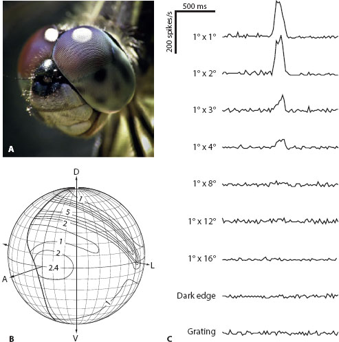
Similar cells to the SF-STMDs of flies are also found in the dragonfly brain, not for spotting females but for spotting prey. These insects have among the best-developed dorsal acute zones found in apposition eyes (figure 6.11A,B), with values of Δφ falling to an incredibly low 0.24° in Anax junius (Sherk, 1978). The facet diameters here are huge (62 μm), and this, together with a yellow screening pigment between the ommatidia, which is transparent to the light that reconverts rhodopsin (Labhart and Nilsson, 1995), helps to ensure high sensitivity. The acute zone—clearly visible even to our own naked eye (figures 6.6D and 6.11A)—has its region of highest resolution distributed in an elongated dorsal strip (figure 6.11B). And just as in male flies, this region eventually feeds its high resolution and sensitivity to large specialized cells in the brain, which behave as matched filters for fly-sized prey objects against a bright background (figure 6.11C: see Olberg, 1981, 1986; O’Carroll, 1993; see also chapter 10). In the large Australian dragonfly Hemicordulia tau, the CSTMD4 cell, a large-field small-target-detecting cell from the lobula, has a response that is tuned to very small moving targets (figure 6.11C), around 1 square degree in size (or even less, as recent recordings indicate). When the target size increases, the response of CSTMD4 drops dramatically. Another set of neurons—eight pairs of target-selective descending neurons (TSDNs) located in the brain—use the information processed by cells like CSTMD4 to calculate a continuously updated mean vector to the target and alter the dragonfly’s flight path accordingly, thus allowing it to “lock onto” and eventually intercept the prey being pursued (Gonzalez-Bellido et al., 2013).
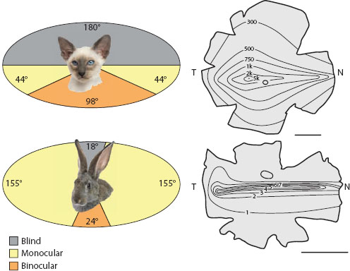
The large flattened forward-facing eyes of praying mantises (Kral, 1999) and long-legged flies (figure 6.6B), or the highly resolved principal eyes of jumping spiders (figure 6.4), are further examples of invertebrate eyes that possess well-developed acute zones for hunting. The pressures of hunting, or being hunted, are even detectable in the eyes of vertebrates. A classic example is seen in the placement and visual fields of the two eyes (figure 6.12). Predators such as cats, foxes, and owls typically have their eyes placed frontally on the head, each eye sharing a very large part of the visual field of the other (Walls, 1942; Hughes, 1977). This large “binocular overlap”—which in cats occurs over 98° of the frontal visual field—is an important requirement for stereopsis, the ability to discriminate depth, that is, to calculate the distance to objects in three-dimensional space. To be a successful predator it is probably highly beneficial to have good stereopsis in the frontal visual field in order to judge the distance to prey during pursuit and to adjust pursuit and interception tactics accordingly. The price paid for this benefit is the large part of the world that remains invisible—in cats, this region is half of all visual space, the 180° of the world that lies directly behind them. Some predators compensate for this loss by being able to turn their heads. Many owls, for instance, can turn their heads by up to 270°!
Rabbits and woodcock, in contrast, are classic prey animals, with laterally placed eyes possessing a panoramic view of the world with a minimal blind spot (Hughes, 1977). Usually rather sedentary, these animals scan the 360° horizon around them, constantly on the lookout for cursorial predators. In rabbits this has resulted in a remarkable matched filter for sampling the full arc of the horizon (figure 6.12)—a so-called horizontal “visual streak” of high ganglion cell density (and high spatial resolution). Even in cats, which need most of their resolving power in the frontal direction, a weak horizontal streak is evident. This is not so surprising—their prey, after all, are also constrained to the same horizon.
Figure 6.11 The dorsal acute zone of dragonflies. (A) An unknown species of dragonfly with eyes possessing distinct dorsal acute zones with larger facet lenses. (Photo credit: Tanya Consaul: 123RF.com photo agency) (B) Map of spatial resolution in the eye of the dragonfly Anax junius (expressed as the number of ommatidial axes per square degree). Density of ommatidia (and thus spatial resolution) increases rapidly in the dorsal (D) visual field. V = ventral, L = lateral, A = anterior. (Redrawn from Land and Nilsson, 2012, with data from Sherk, 1978) (C) Responses (peristimulus time histograms) of CSTMD4, a large-field small-target-detecting cell from the lobula of the dragonfly Hemicordulia tau. In the part of the cell’s receptive field corresponding to its dorsal acute zone the cell is most sensitive to small, dark, and reasonably slow-moving targets (as a fly might appear during a highly fixated pursuit). It is insensitive to large bars, edges, and gratings. (From O’Carroll, 1993, reprinted with permission from Macmillan Publishers Ltd.)
Of course, the horizon—and the great variety of visually important events that are constrained there—have not only led to the evolution of visual streaks in predators and prey. In fact horizontal visual streaks are common in all types of animals that inhabit flat environments (Hughes, 1977). Indeed, the spatial layout of animal habitats—whether flat or highly complex—has profoundly influenced the way the eye’s sampling matrix has evolved.
Figure 6.12 Visual fields of predators and prey. Cats (upper panels) have receptive fields typical of predators with frontally directed eyes, a large 180° blind spot to the rear, and large frontal binocular overlap for accurate distance estimations during prey pursuit. A temporal fovea and a mild visual streak (seen as a ganglion cell density map in cells/mm2 on a flattened corneal mount) emphasize the importance of a frontally directed gaze coupled with enhanced prey detection around the horizon. Rabbits, in contrast (lower panels), are typical of prey animals, with about 340° of surround vision, a small rear blind spot, and modest frontal binocular overlap. Their ganglion cell maps (in thousands of cells/mm2) reveal a highly developed horizontal visual streak for optimal predator detection around the horizon. N = nasal, T = temporal. Scale bars = 10 mm. (All panels created using data in Hughes, 1977. Photo credits: Oleg Zhukov and Eric Isselee: 123RF. com photo agency)
The Physical Layout of Terrestrial Habitats
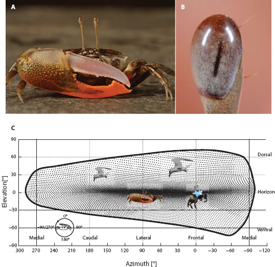
A horizontal visual streak is a common feature in the apposition compound eyes of insects and crustaceans inhabiting flat environments such as open featureless deserts (e.g., desert ants), water surfaces (e.g., water striders), and intertidal mud flats (e.g., fiddler crabs). The tall barrel-shaped eyes of fiddler crabs are particularly extreme in this respect (figure 6.13; Zeil and Hemmi, 2006; Smolka and Hemmi, 2009). Every thing in the life of a fiddler crab is defined by the single dominating feature of its extremely flat habitat—the horizon. This fact manifests itself in the way the eyes are constructed. Not only does each eye sample the entire 360° arc of the horizon, over one third of all ommatidia have their fields of view crammed into the narrow strip of space that corresponds to this single feature (figure 6.13C). The horizon is thus sampled very finely as well as panoramically. Because the corneal surface is much flatter in the dorsal direction than the horizontal, the eye samples vertical space (Δφv) much more finely than horizontal space (Δφh). In the acute zone Δφv falls to around 0.3°—at the same location Δφh is about 1° larger. This optical arrangement breaks up the eye into three main zones—a dorsal zone, a highly resolved equatorial zone, and a ventral zone. Each of them has a special ecological significance, more or less functioning as a matched filter for a specific set of tasks. Anything seen above the line of the horizon in the dorsal zone is interpreted as a predator and induces the crab to make a rapid retreat to its burrow. Anything seen equatorially is interpreted as a conspecific, either a mate or a rival, whereas anything seen in the ventral zone implies the close proximity of a conspecific and the possibility for the discrimination of social signals (Smolka and Hemmi, 2009).
Figure 6.13 Horizontal acute zones in compound eyes. (A) Male fiddler crab Uca vomeris, with the large right claw typical of its sex and two prominent eye stalks. (Photo courtesy of Jeff Wilson) (B) The tall cylindrical eye, which is up to 2.3 mm high and 1.4 mm wide. (Photo courtesy of Ajay Narendra) (C) The optical axes of all ommatidia in the compound eye (black dots), where the edge of the eye’s visual field is shown as a thick dark line. Insets show relevant behavioral tasks in specialized areas: individual recognition frontally (female carapace pattern), burrow defense laterally (male with large claw), and predator avoidance dorsally (terns). (From Smolka and Hemmi, 2009, with kind permission of the Company of Biologists)
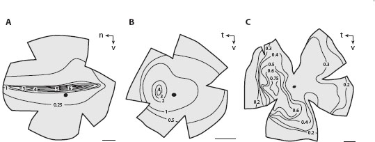
Figure 6.14 Habitat-related ganglion cell topographies in terrestrial mammals. Ganglion cell densities are given in thousands of cells/mm2 (all other conventions as in figure 6.12). (A) The red kangaroo Megalia rufa, with a distinct horizontal visual streak. (B) Doria’s tree kangaroo Dendrolagus doriana, with no obvious retinal specialization. (C) The two-toed sloth Choloepus didactylus, with a vertical visual streak. V = ventral; scale bar = 5 mm. (From Collin, 1999, with references therein, reprinted with kind permission from Springer Science+Business Media)
Vertebrates also show a similar response to the horizon. Rabbits, as we have seen, have a horizontal visual streak of increased ganglion cell density (figure 6.12). So do many fish that inhabit broad flat sandy seafloors, such as the red-throated emperor and several species of benthic sharks (Collin and Pettigrew, 1988; Lisney and Collin, 2008). Many animals inhabiting open grassy plains likewise have horizontal visual streaks (Hughes, 1977), such as various ungulates (e.g., cows and deer), elephants, and marsupials. The visual streak of the red kangaroo is particularly distinct (figure 6.14A), but in tree kangaroos it is completely absent (figure 6.14B). This large difference in retinal design is directly related to habitat, a fact that led Austin Hughes to develop his “terrain theory” of vision (Hughes, 1977): the physical layout of sampling stations in a retina reflects the physical structure of the animal’s normal habitat. In the case of the red kangaroo, which inhabits open plains that are dominated by the horizon, a horizontal visual streak was the evolutionary response to this particular “terrain.” For tree kangaroos, where the horizon is obscured by a complicated three-dimensional habitat full of trees and vines, and where no single feature dominates, the evolutionary response to this “terrain” has instead been a circularly concentric gradient of ganglion cell density. Interestingly, another tree dweller, the two-toed sloth, instead has a vertical visual streak (figure 6.14C). This it possibly uses to align its head with the branch from which it hangs upside down.
The Physical Layout of Aquatic Habitats
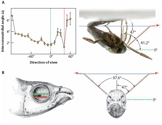
As we saw in chapter 2, the optical properties of water have important consequences for aquatic visual environments. With increasing depth, the color, intensity, polarization, and directionality of light change dramatically, and depending on water clarity—which may vary quite significantly from one body of water to another—the veiling haze of scattered space light may be more or less pronounced. All of these properties have had major affects on the evolution of spatial sampling in the eyes of aquatic animals. The same is true of the optical properties of the water surface itself. The fact that water has a higher refractive index than air means that the entire 180° dome of the world above the water surface is compressed to a 97.6° cone of light under water. Within this cone of light—called “Snel’s window”—all the features of the terrestrial world above can be found, including the flat water surface, which is located at the edge of the cone (chapter 2; Walls, 1942, p. 378). By looking upward along the edge of the cone, an animal just below the water surface would have a periscopic view of the water surface above and see anything, including prey, that might be trapped on it. One such animal is the backswimmer Notonecta glauca, which stalks prey on the water surface while suspended underneath. The water surface is an important horizon for the backswimmer, and the ventral part of the eye possesses a well-developed visual streak (figure 6.15A) that watches the surface along the edge of Snel’s window (Schwind, 1980). This matched filtering does not stop at the optics of the eye: in the optic lobe there are cells that have their visual fields coincident with the visual streak and that respond maximally to prey-sized objects on the water surface (Schwind, 1978). But the water surface is not the backswimmer’s only horizon. Frontward, the backswimmer can also see the environment of the pond and any item of interest that might be located there. There is a second visual streak that views this direction as well (Schwind, 1980)! Remarkably, exactly the same type of visual adaptation has convergently evolved in the surface-feeding fish Aplocheilus lineatus (figure 6.15B), whose camera eyes also have two visual streaks, one viewing the boundary of Snel’s window, the other looking into the water horizontally. As we noted earlier, horizontal visual streaks can also be found in several species of benthic fish and sharks. .
As one descends deeper in the open ocean, the dramatic decline of light intensity and its increasingly dorsal direction of incidence have a profound affect on the nature of the visual scene encountered at different depths. In terrestrial habitats visual scenes are said to be “extended”; that is, light reaches the eye from many different directions at once. Nonetheless, terrestrial animals also experience sources of light that are much smaller in spatial extent. Stars, for instance, are point sources. So too are the flashes of bioluminescence produced by nocturnal fireflies. The tiny dark silhouette of a female fly passing across a bright sky will also be point-like to a male fly in hot pursuit. However, it is within the depths of the sea that this distinction between extended sources and point sources has its greatest influence on the visual systems of animals. In the shallower depths, where scattered daylight produces an even blue space light and where the sea floor may be clearly visible, visual scenes are extended in all directions. But at greater depths, where the space light is diminished, bioluminescent point sources also begin to appear, especially from below, where the space light is up to 300 times dimmer than that coming from above. Upward and even laterally, the scene is still extended. But downward the scene begins to be dominated by point sources. At still deeper levels bioluminescent point sources can be seen in all directions. In these mesopelagic depths between 200 m and 1000 m, the scene is semiextended, becoming less extended and more point-like as the space light diminishes with increasing depth. Below 1000 m, where daylight no longer penetrates, the visual scene is entirely point-like in nature.
Figure 6.15 Vision through Snel’s window, where the 180° view of the world above the water surface is compressed by refraction into a 97.6°-wide cone below the water surface. (A) The backswimmer Notonecta glauca hangs upside down at the water surface, with the ommatidia in the ventral regions of its apposition eyes looking upward (positive directions of view in the left panel). At precisely the boundary of Snel’s window (red dashed lines), there is a sudden decrease in Δφ indicating enhanced spatial resolution for objects (prey) on the horizontal water surface above. In the horizontal direction below the water surface (0°: green dashed lines) Δφ is also minimal, indicating the presence of a second horizontal acute zone. (B) Two horizontal visual streaks are also found in the surface-feeding fish Aplocheilus lineatus, one for the horizontal water surface above (red dashed lines) and one for the horizontal underwater world around it (green dashed lines). (Adapted from Wehner, 1987, with kind permission from Springer Science+Business Media, with data and images from Schwind, 1980, and Munk, 1970. Photo credit: Eric Isselee: 123RF.com photo agency)
Not surprisingly, the eyes of deep-sea animals have evolved in response to this changing nature of visual scenes with depth, being optimized for dim extended day-light or for the detection of bioluminescent point sources or both (Warrant, 2000; Warrant and Locket, 2004). As we saw in chapter 4, to accurately localize a narrow point of bioluminescence in the darkness of the deep sea requires another type of eye design than that which is optimal for a dim extended scene. The image of a point source on the retina is, by definition, also a point of light (assuming that aberrations and diffraction do not blur the image too much). For a visual detector to collect all the light from this point, its receptive field need not be any larger than the image itself. Receptors viewing large solid angles of space or performing spatial summation—so important for improved sensitivity to a dim extended scene (see chapter 11)—are useless for improving detection of a point source. In fact, one would predict that eyes built to see point sources of light against a dark background should have (1) a wide pupil to collect sufficient photons to detect the point source (equation 4.1c) and (2) good spatial resolution to then accurately localize it. This is precisely what one sees in the eyes of deep-sea fish as one goes deeper in the ocean, from the dim extended world of the mesopelagic zone to the dark point-source world of the bathypelagic zone (figure 6.16A; Warrant, 2000; Warrant and Locket, 2004).
Consider a plot of the smallest angular separation of ganglion cells as a function of depth for some 20 species of deep-sea fish (figure 6.16A). A smaller separation of ganglion cells results in a greater anatomical resolution. Two trends are obvious. First, the eyes of fish on average become sharper with depth, with the eyes of bathypelagic fish being the sharpest, typically having the potential to resolve details subtending just 5 minutes of arc. This is perfect for detecting point-source bioluminescence, the only light source at these depths. Second, the variation across species in ganglion cell separation (and thus resolution) is large in the brighter upper levels (figure 6.16A: error bars) but gradually declines with depth, with minimal variation in the bathypelagic zone (separation = 4.8 ± 2.9 arc minutes). The small variation in the bathypelagic zone is easy to understand: here the only light sources are point sources, and the best strategy involves little summation and high resolution. The large variation in the mesopelagic zone reflects its semiextended nature, with some species adapted to point sources, some to extended sources, and others to both (Warrant, 2000). The bathypelagic Rouleina attrita (figure 6.16B) well exemplifies the trend toward sharp vision at depth. Living near sea floors between 1.4 and 2.1 km below the sea surface (Wagner et al., 1998), Rouleina has sharp frontally directed deep convexiclivate foveae possessing up to 27,000 ganglion cells/mm2, giving them a resolution of around 5 minutes of arc. The same arguments apply to dorsally directed eyes that accurately detect the small dark silhouettes of other animals in the dim downwelling daylight. The large apposition eyes of hyperiid amphipods (Land, 1989b, 2000) and the superposition eyes of euphausiids (Land et al., 1979) become increasingly dorsal in their field of view—and increasing well resolved—with increasing depth.
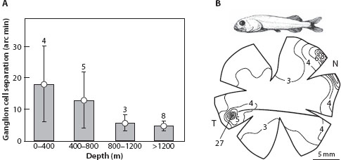
Figure 6.16 Deep-sea eye structure and the changing nature of visual scenes with depth. (A) The finest separation of ganglion cells found in a survey of 20 species of deep-sea fish living at different depths, showing mean separation (in arc minutes) ± SD (with number of included species indicated above each histogram bar). Deeper-living fish tend toward sharper retinas, a reflection of the increasing dominance of bioluminescent point-source illumination with depth. (B) Rouleina attrita has a retinal design that is common in bathypelagic fish, with deep convexiclivate temporal foveae containing densely packed ganglion cells (in thousands of cells/mm2). This design is ideal for localizing bioluminescent point sources in the frontal visual field. (From Warrant, 2000, with data from Wagner et al., 1998)
Near the surface, where scenes are as extended as they are on land, the evolutionary pressures on spatial vision are very similar to those in terrestrial habitats. What varies more rapidly with depth, however—even in the shallows—is the spectrum of natural daylight. This, it turns out, has also had a significant effect on the evolution of vision—particularly with regard to the perception of color, the topic to which we turn next.