CHAPTER 9

Amplification of Light. Lasers

9.1 Introduction

Few developments have produced an impact on any established field of science compared to the effect of the laser or optical maser20 on the field of optics. Vacuum-tube oscillators that generate coherent electromagnetic radiation at frequencies up to about 10⁹ Hz have been known for many years. In 1954 the maser was developed [13]. The maser generates microwaves (10⁹ to 10¹¹ Hz). The practical feasibility using the maser principle for the amplification of light (∼ 10¹⁴ Hz) was studied in 1958 by Schawlow and Townes who laid down the basic theoretical groundwork. The first working laser, made of synthetic ruby crystal, was produced in 1960 at the Hughes Research Laboratories. It was followed in a few months by the helium—neon gas laser developed at the Bell Telephone Laboratories. The ruby laser generates visible red light. The helium—neon laser generates both visible red light and infrared radiation. Since their introduction, numerous types of lasers have been produced that generate radiation at various optical frequencies extending from the far infrared to the ultraviolet region of the spectrum [25].

A laser is basically an optical oscillator. It consists essentially of an amplifying medium placed inside a suitable optical resonator or cavity. The medium is made to amplify by means of some kind of external excitation. The laser oscillation can be described as a standing wave in the cavity. The output consists of an intense beam of highly monochromatic radiation.

Conventional light sources (arcs, filaments, discharges) provide luminous intensities corresponding to thermal radiation at temperatures of no more than about 10⁴ °K. With lasers, intensities corresponding to 10²⁰ to 10³⁰ degrees are readily attained. Such enormous values make possible the investigation of new optical phenomena such as nonlinear optical effects, optical beating, long-distance interference, and many others that were previously considered out of the question. Practical applications of the laser include long-distance communications, optical radar, microwelding, and eye surgery, to mention only a few.

9.2 Stimulated Emission and Thermal Radiation

Einstein in 1917 first introduced the concept of stimulated or induced emission of radiation by atomic systems. He showed that in order to describe completely the interaction of matter and radiation, it is necessary to include that process in which an excited atom may be induced, by the presence of radiation, to emit a photon, and thereby decay to a lower energy state.

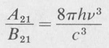
Consider a quantized atomic system in which there are levels labeled 1,2,3, ... , with energies E₁, E₂, E₃, and so forth. The populations, that is, the number of atoms per unit volume, in the various levels, are N₁, N₂, N₃, and so forth. If the atomic system is in equilibrium with thermal radiation at a given temperature T, then the relative populations of any two levels, say 1 and 2, are given by Boltzmann’s equation

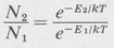
(9.1)

where k is Boltzmann’s constant. If we assume, for definiteness, that E₂ > E₁, then N₂ < N₁.

An atom in level 2 can decay to level 1 by emission of a photon. Let us call A₂₁ the transition probability per unit time for spontaneous emission from level 2 to level 1. Then the number of spontaneous decays per second is N₂A₂₁. [The value of A₂₁ can be calculated from Equation (8.8) of the previous chapter.]

In addition to these spontaneous transitions, there will be induced or stimulated transitions. The total rate of these induced transitions between level 2 and level 1 is proportional to the energy density u_v of the radiation of frequency v, where

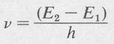
(9.2)

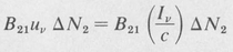
Let B₂₁ and B₁₂ denote the proportionality constants for stimulated emission. Then the number of stimulated downward transitions (emissions) per second is

N₂B₂₁ u_v

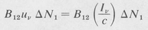
Similarly, the number of stimulated upward transitions (absorptions) per second is

N₁B₁₂ u_v

The proportionality constants in the above expressions are known as the Einstein A and B coefficients.

Under equilibrium conditions the net rate of downward transitions must be equal to that of upward transitions, namely,

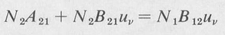
(9.3)

By solving for u_v, we obtain

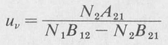
Further, in view of Equation (9.1), we can write

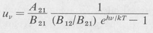
(9.4)

In order for this to agree with the Planck radiation formula, the following equations must hold:

(9.5)

(9.6)

Thus for atoms in equilibrium with thermal radiation, the ratio of stimulated emission rate to spontaneous emission rate is given by the formula

(9.7)

We recall from Section 7.5 that this is precisely the same as the number of photons per mode, that is, the occupation index.

According to the above result, the rate of induced emission is extremely small in the visible region of the spectrum with ordinary optical sources (T ∼ 10³ °K). Hence, in such sources most of the radiation is emitted through spontaneous transitions. Since these transitions occur in a random manner, ordinary sources of visible radiation are incoherent.

On the other hand, in a laser the radiation density for certain preferred modes builds up to such a large value that induced transitions become completely dominant. One result is that the emitted radiation is highly coherent. Another is that the spectral radiance at the operating frequency of the laser is vastly greater than that of ordinary light sources.

9.3 Amplification in a Medium

Consider an optical medium through which radiation is passing. Suppose that the medium contains atoms in various energy levels, E₁ E₂, E₃, and so forth. Let us fix our attention on two levels, say E₁ and E₂, where E₁ < E₂. We have already seen that the rates of stimulated emission and absorption involving these two levels are proportional to N₂B₂₁ and N₁B₁₂, respectively. Since B₂₁ = B₁₂, the rate of stimulated downward transitions will exceed that of upward transitions if

N₂ > N₁

that is, if the population of the upper state is greater than that of the lower state.21

Such a condition is contrary to the thermal equilibrium distribution given by the Boltzmann equation (9.1). It is called a population inversion (Figure 9.1). If a population inversion exists, then, as we shall show, a light beam will increase in intensity or, in other words, it will be amplified as it passes through the medium. This is because the gain due to the induced emission exceeds the loss due to absorption.

Figure 9.1. Graphs of the population densities of two levels of a system. (a) Normal or Boltzmann distribution; (b) inverted distribution.

The induced radiation is emitted in the same direction as the primary beam and it also has a definite phase relationship; that is, it is coherent with the primary radiation. This can be argued on the basis of the modes of the electromagnetic radiation field. The act of stimulated emission of a single atom results in the addition of a photon to the particular mode that causes the stimulated emission. As we have shown, the rate of stimulated emission is proportional to the number of photons in the mode in question. Modes are distinguished from one another by frequency, direction of the wave vector, and polarization. Hence a photon that has been added to a given mode by stimulated emission is a copy of the photons that are already in that mode.

The Gain Constant In order to determine quantitatively the amount of amplification in a medium, we must take a closer look at the details of emission and absorption. Suppose a parallel beam of light propagates through a medium in which there is a population inversion. For a collimated beam, the spectral energy density u_v is related to the spectral irradiance I_v in the frequency interval v to v + ∆v by the formula

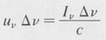
(9.8)

Due to the Doppler effect and other line-broadening effects, not all of the atoms in a given energy level are effective for emission or absorption in a specified frequency interval. Rather, a certain number per unit volume, say ∆N₁, of the N₁ atoms per unit volume in level 1, is available. Consequently, the rate of upward transitions is

Similarly, the rate of induced downward transitions is

Now each upward transition subtracts a quantum of energy hv from the beam. Similarly, each downward transition adds the same amount. Therefore the net time rate of change of the spectral energy density in the interval ∆v is given by

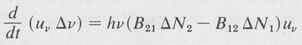
(9.9)

In time dt the wave travels a distance dx = c dt. Hence, in view of Equation (9.8) we can write

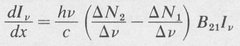
(9.10)

giving the rate of growth of the beam in the direction of propagation.

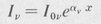
The above differential equation can be integrated to give

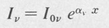
(9.11)

in which α_v is the gain constant at frequency v. It is given by

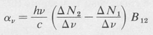
(9.12)

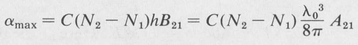
An approximate expression for the gain constant at the center of a spectral line is obtained by taking ∆v to be the linewidth. The ∆Ns are then set equal to the Ns. The result, which is correct except for a numerical constant of the order of unity, is

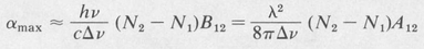
(9.13)

The last step follows from the relation between the Einstein A and B coefficients, Equation (9.6).

We see that α is positive if N₂ > N₁, which is the condition for amplification. Otherwise, if N₂ < N₁ (which is the normal equilibrium condition), then α is negative and we have absorption. Methods for producing population inversions in optical media will be discussed in the following section.

The Gain Curve In order to determine how the gain varies with frequency, it is necessary to consider the details of line broadening. In the case of broadening due to thermal motion alone, elementary kinetic theory [31] gives the fraction of atoms whose x component of velocity lies between u_x and u_x + ∆u_x. This fraction is a Gaussian function, namely,

in which C = (ml2πkT)^½ and a = m/2kT. Here T is the absolute temperature and k is Boltzmann’s constant. Due to the Doppler effect, these atoms will emit or absorb radiation, propagating in the x direction, of slightly different frequency v than the resonance frequency v₀ of the atom when it is at rest. The frequency difference is given by

It follows that the number of atoms in a given level that can absorb or emit in the frequency range v to v + ∆v is given by

in which β = mc²/(2kTv₀²). This can be substituted for ∆N₁ and ∆N₂ in Equation (9.12). The result is

(9.14)

Thus the gain for a Doppler broadened laser transition varies with frequency according to a Gaussian function. A curve is shown in Figure 9.2. This same curve also represents the profile of a Doppler-broadened spectral line. The maximum gain occurs at the line center and is given by

(9.15)

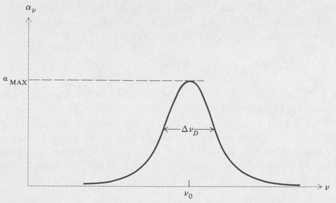
Figure 9.2. Amplification coefficient for a Doppler broadened spectral line.

In order to compare this with the approximate value expressed by Equation (9.13) we must calculate the width of a Doppler-broadened line. The width at half maximum is found by setting the exponential factor equal to , that is, v — v_o = (In 2/β)^½. Twice this value is the full width ∆v_D = 2(ln 2/β)^½. On using the definitions of C and β given above, we readily find

(9.16)

The numerical factor 2(ln 2/π)^½ = 0.939, hence the previous formula (9.13) is quite accurate in this case.

9.4 Methods of Producing a Population Inversion

There are several methods for producing the population inversions necessary for optical amplification to take place. Some of the most commonly used are

1. Optical pumping or photon excitation
2. Electron excitation
3. Inelastic atom—atom collisions
4. Chemical reactions

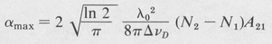
In the case of optical pumping, an external light source is employed to produce a high population of some particular energy level in the laser medium by selective optical absorption [Figure 9.3(a)]. This is the method of excitation used in the solid-state lasers of which the ruby laser is the prototype.

Figure 9.3. Diagrams showing three processes for producing a population inversion. (a) Optical pumping; (b) direct electron excitation; (c) inelastic atom—atom collisions.

Direct electron excitation in a gaseous discharge may be used to produce the desired inversion [Figure 9.3(b)]. This method is used in some of the gaseous ion lasers such as the argon laser. With this type of excitation the laser medium itself carries the discharge current. Under suitable conditions of pressure and current, the electrons in the discharge may directly excite the active atoms to produce a higher population in certain levels compared to lower levels. The relevant factors are the electron excitation cross section and the lifetimes of the various levels.

In the third method, an electric discharge is also employed. Here a suitable combination of gases is employed such that two different types of atoms, say A and B, both have some excited states, A* and B*, that coincide, or nearly coincide. In this case transfer of excitation may occur between the two atoms as follows:

A* + B → A + B*

If the excited state of one of the atoms, say A*, is metastable, then the presence of gas B will serve as an outlet for the excitation. As a consequence it is possible that the excited level of atom B may become more highly populated than some lower level to which the atom B can decay by radiation [Figure 9.3 (c)]. This is the case with the helium—neon laser. A neon atom receives its excitation from an excited helium atom. The laser transition then occurs in the neon atom.

The fourth method defines a class of lasers known as chemical lasers. Here a molecule is caused to undergo a chemical change in which one of the products of the reaction is a molecule, or an atom, that is left in an excited state. Under appropriate conditions a population inversion can occur. An example is the hydrogen fluoride chemical laser in which excited hydrogen fluoride molecules result from the reaction

H₂ + F₂ → 2HF

9.5 Laser Oscillation

The optical cavity or resonator of a laser usually consists of two mirrors, curved or plane, between which the amplifying medium is located (Figure 9.4). If a sufficient population inversion exists in the medium, then the electromagnetic radiation builds up and becomes established as a standing wave between the mirrors. The energy is usually coupled from the resonator by having one or both of the mirrors partially transmitting.

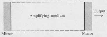
Figure 9.4. Basic laser setup.

In the case of plane reflectors, the optical cavity is similar to a conventional Fabry-Perot interferometer. The pass bands of the Fabry-Perot resonator occur at an infinite number of equally spaced frequencies

. . . , v_n, v_n+1, v_n+2, . . .

They differ by the free spectral range

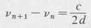
where c is the speed of light and d is the spacing of the reflectors. These frequencies define what are known as the longitudinal modes of the resonator. There are also transverse modes, as discussed in the following section.

Oscillation may occur at one or more of these resonant frequencies, depending on the width of the gain curve in relation to the mode spacing (Figure 9.5). Most lasers oscillate on several modes at once.

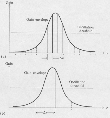
Figure 9.5. Oscillation frequencies in a laser. (a) Four longitudinal modes; (b) one mode.

If extremely high spectral purity is needed, however, it is possible to obtain oscillation on one mode by suitable selection of laser parameters. The inherent linewidth in this case is determined mainly by the quality factor Q of the laser resonator. These linewidths are typically of the order of a few hertz. However, in practice, linewidths of the order of 10³ Hz are obtained. The limitation is determined largely by mechanical and thermal stability.

Threshold Condition for Oscillation We have seen that the irradiance of a parallel beam in an amplifying medium grows according to the equation

Suppose a wave in a laser cavity starts out at some point and travels back and forth between the cavity mirrors. On its return the wave will lose a certain fraction δ of its energy by scattering, reflection loss, and so forth. In order for the laser to oscillate, the gain must equal or exceed the loss, that is,

I_v — I_0v ≥ δI_v

or, equivalently,

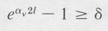
(9.17)

Here l is the active length of the amplifying medium. If α_v2l ≪ 1, then the condition for oscillation can be written

(9.18)

If at a given frequency the gain exceeds the loss, the ensuing oscillation grows until an equilibrium condition is attained. The fractional loss δ is essentially constant and independent of the amplitude of the oscillation. Hence a depletion of the medium occurs that diminishes the population difference N₂ — N₁. The gain then drops until

(9.19)

The depletion occurs in a band centered on the oscillation frequency and is called hole burning. The shape of the hole is an inverted resonance curve, similar to the resonance curve of a harmonic oscillator known as a Lorentz profile. The width of the Lorentz profile is equal to the reciprocal of the radiative lifetime of the lasing atom. If this radiative width is as large or larger than the width of the gain curve, then all of the excited atoms can be said to be “in communication with” the oscillating laser mode in question. This situation is termed homogeneous broadening. On the other hand if the radiative width of the laser transition is smaller than the width of the gain curve, then only part of the atoms participate in a given mode. This is called inhomogeneous broadening. In this case hole burning results in a modification of the gain curve as shown in Figure 9.6.

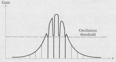
Figure 9.6. Hole burning of the gain envelope in a laser.

9.6 Optical-Resonator Theory

The concept of spatial modes of electromagnetic radiation in a closed cavity was briefly discussed in Section 7.3. There it was shown that a given mode can be specified by three integers that are directly related to the standing-wave pattern of the mode in question. In the case of a laser resonator, the cavity is not closed, being formed by only two reflecting surfaces. However, such open-sided resonators can still support a three-dimensional standing wave, sometimes referred to as a “quasi mode.” One important fact is that part of the energy “spills” around the reflecting mirrors and is lost. This is called the diffraction loss of the resonator. A careful examination of such losses is necessary in laser applications, especially for low-gain systems such as the helium—neon laser in which the amplification per pass is typically only a few percent.

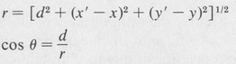
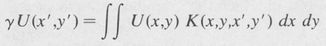
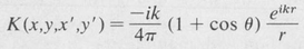
To illustrate the mathematical problem involved in the study of the optical resonator, we show in Figure 9.7 the resonator mirrors with aperture coordinates x,y and x’ ,y’, respectively. The case is equivalent to diffraction with multiple apertures, as shown. If U (x,y) and U‘(x’,y’) represent the complex amplitudes of the radiation over the mirror surfaces, then by applying the Fresnel-Kirchhoff diffraction theory (Section 5.2) we can write

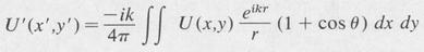
(9.20)

in which

If the mirrors are identical, which is typical, then for the steady state condition, that is, after the radiation has been reflected back and forth many times, the two functions U and U’ will become identical, except for a constant factor γ. In this case

(9.21)

where

(9.22)

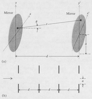
Figure 9.7. (a) Geometry of a Fabry-Perot laser cavity; (b) equivalent multiple diffraction problem.

Equation (9.21 ) is an integral equation in the unknown function U. The function K is called the kernel of the equation, and γ is known as the eigenvalue. There are an infinite number of solutions U_n, n = 1,2, ... , each with an associated eigenvalue γ_n. The various solutions correspond to the normal modes of the resonator. Expressing γ_n as

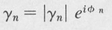
(9.23)

we see that |γ_n| specifies the ratio of the amplitude, and φ_n gives the phase shift associated with a given mode. The quantity 1–|γ_n|² is the relative energy loss per transit due to diffraction. (This is in addition to losses caused by absorption by the mirrors.)

Fox and Li were among the first to study the integral equation of the Fabry-Perot resonator [9]. They employed an electronic digital computer to find numerical solutions and associated eigenvalues. Boyd and Gordon found analytical solutions [6]. The types of optical resonators studied included both plane-parallel mirrors and curved mirrors.

Although accurate solutions of the Fabry-Perot resonator problem are quite involved, it is possible to find a simple approximation by employing the same procedure as that of the Fraunhofer diffraction case. Equation (9.22) then reduces to

K(x,y,x’,y’) = Ce^{-ik1(xx’ + yy’)}

in which, under the approximation cited, C and k₁ are constants. The integral equation (9.21 ) then becomes

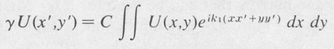
(9.24)

This equation says that the function U(x,y) is its own Fourier transform. The simplest of such functions is the Gaussian

(9.25)

Here w is a scaling constant, and ρ² = x² + y². More general functions that are their own Fourier transforms are products of functions known as Hermite polynomials [27] and the Gaussian above, namely,

(9.26)

The integers p and q denote the order of the Hermite polynomials,²² and each set (p,q) corresponds to a particular transverse mode of the resonator.

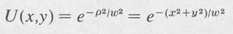
The lowest-order Hermite polynomial H_o is a constant, namely, unity, hence the simple Gaussian mode corresponds to the set (0,0) and is called the TEM₀,₀ mode. The terminology TEM refers to the transverse electromagnetic waves in the cavity. Sometimes the notation TEM_n,p,q is used, where the integer n is the longitudinal-mode number, and p and q are the transverse-mode numbers. Some low-order mode patterns are illustrated in Figure 9.8.

Figure 9.8. Field distributions at the mirrors for some low-order modes.

Resonator Configurations. Stability There are many combinations of curved and plane mirrors that can be used for laser cavities. A few of these are shown in Figure 9.9. One of the most commonly used cavity configurations is known as the confocal resonator. This consists of two identical concave spherical mirrors separated by a distance equal to the radius of curvature. The confocal cavity is very much easier to align than the plane-parallel type. The latter requires an adjustment accuracy of the order of one arc second, whereas the confocal configuration, being somewhat self-aligning, needs a setting accuracy of only about a quarter of a degree in a typical application.

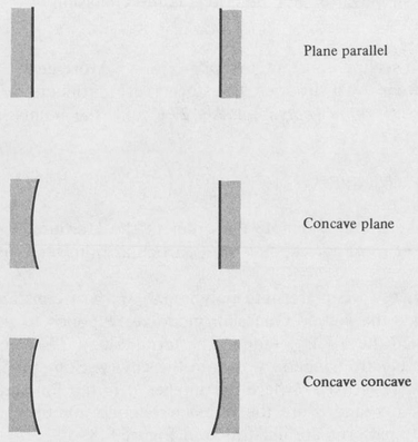
Figure 9.9. Some common laser cavities.

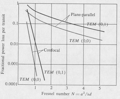
Figure 9.10. Loss curves for the first two modes in plane-parallel and confocal laser cavities.

The diffraction loss, as calculated by Boyd and Gordon, for some of the low-order modes in plane-parallel and confocal resonators is plotted in Figure 9.10. The loss is plotted as a function of the Fresnel number N = a²/λd, where a is the mirror radius and d is the mirror separation. With confocal spherical mirrors, the diffraction losses of low-order modes are negligibly small when N > 1. A comparison of the losses for the plane-parallel resonator and the confocal resonator shows that the latter is definitely superior.

By the use of geometrical optics it is possible to classify laser resonators according to a criterion known as stability. A stable resonator is one in which a ray inside the cavity will remain close to the optic axis upon multiple reflections between the end mirrors. Stability criteria will be derived in the next chapter (Section 10.5). As we shall show, for the symmetrical cavity consisting of two mirrors of the same radius of curvature, the distance of separation must be less than twice the radius of curvature to form a stable cavity.

Spot Size The scale parameter w, introduced in Equations (9.25) and (9.26), is a measure of the lateral distribution of the energy in the optical beam inside the resonator. The Gaussian function falls to e^-1 when ρ, the lateral distance from the optic axis, is equal to w. This function is proportional to the field amplitude; so the energy, being proportional to the square of the field, will fall to e^-2 of its maximum value. Hence w is called the “spot size” of the dominant (0,0) mode.

In a given resonator, w is a function of the longitudinal position. If we call z the longitudinal distance measured from the midpoint between the two mirrors, then, as shown by Boyd and Gordon, the parameter w is given by

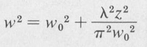
(9.27)

Here λ is the wavelength and W_o is another parameter, namely, the spot size at the center, whose value is determined by the radii of curvature of the mirrors and their separation. For a symmetrical cavity formed by two mirrors each of radius of curvature R and separated by a distance d, the parameter W₀ is given by

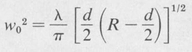
(9.28)

and the radius of curvature of the standing-wave surfaces is given by

(9.29)

In the case of a confocal resonator R = d, we find

for the spot size at the center, and

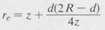
for the spot size at either mirror, z = ±d/2. Figure 9.1 illustrates the confocal case. Surfaces of constant phase are drawn to show the curvature of the standing waves within the cavity. At the mirrors the wave surfaces match the curvature of the mirror surface. At the center, where the spot size is minimum, the wave surface becomes planar. A hemiconfocal cavity would be represented by placing a plane mirror at the center of the confocal cavity, the wave surfaces and spot size remaining unchanged for the portion of the confocal cavity that lies between the mirrors forming the new cavity. In fact, any two wave surfaces will define a cavity if the wave surfaces are replaced by mirrors that match the curvatures of the wave surfaces.

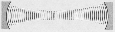
Figure 9.11. Standing wave pattern and lateral distribution of the TEM_0,0 mode of a confocal laser cavity.

9.7 Gas Lasers

Figure 9.12 shows a typical physical arrangement of a gas laser. The optical cavity is provided by external mirrors. The mirrors are coated with multilayer dielectric films in order to obtain high reflectance at the desired wavelength. Spherical mirrors arranged in the confocal configuration are used because of the low loss and ease of adjustment of this type of cavity.

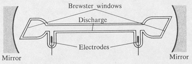
Figure 9.12. Typical design of a gas laser.

The laser tube is fitted with Brewster end windows in order to obtain the maximum possible transparency. When Brewster windows are used, the output of the laser is linearly polarized. The reason is that the windows are highly transparent for one preferred direction of polarization—the TM polarization—as discussed in Section 2.8. Consequently, laser oscillation at this favored polarization builds up and becomes dominant over the orthogonal TE polarization.

External electrical excitation may be provided in any of the following ways:

1. Direct-current discharge
2. Alternating-current discharge
3. Electrodeless high-frequency discharge
4. High-voltage pulses

Methods (1) and (2) are commonly employed in commercial gas lasers. The direct-current discharge ( 1 ) is advantageous if the laser is to be used for such things as optical heterodyning, communications, and so forth. The alternating-current discharge (2) is simplest because the power source need be only an ordinary high-voltage transformer connected to cold metal electrodes in the tube. The electrodeless high-frequency discharge (3) was used in the first gas laser—the helium—neon laser—developed at the Bell Telephone Laboratories by Javan, Bennett, and Herriott [21]. Method (4) is employed in many high-power pulsed lasers and is necessary in some instances in which a steady population inversion cannot be maintained.

The Helium—Neon Laser Figure 9.13 shows an energy-level diagram of the helium—neon laser system. Helium atoms are excited by electron impact in the discharge. The populations of the metastable states ³S and ¹S of helium build up because there are no optically allowed transitions to lower levels. It is seen from the figure that the neon levels labeled 2s and 3s lie close to the metastable helium levels.

Figure 9.13. Simplified energy-level diagram of the helium—neon laser.

There is, therefore, a high probability of energy transfer when a metastable helium atom collides with an unexcited neon atom. These energy transfers are

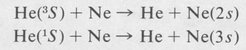
Under suitable discharge conditions a population inversion of the Ne(2s) and Ne(3s) levels can take place. The optimum value of total pressure is about 1 torr, and the most favorable ratio of helium to neon is found to be about 7: 1.

The main laser action in the helium—neon system corresponds to the following transitions in the neon atom:

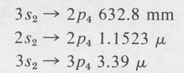
In addition to these, many weaker transitions in neon have been made to undergo laser oscillation [25].

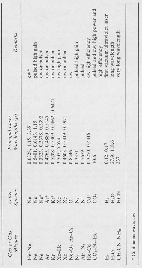
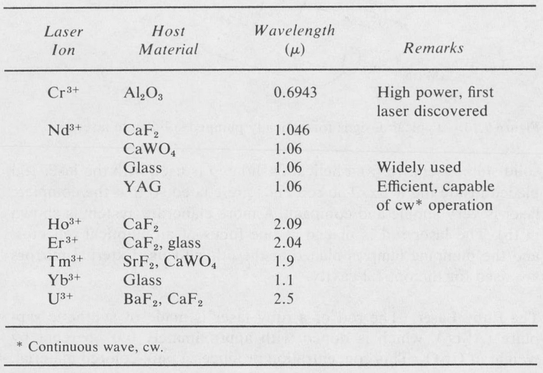
Other Gas Lasers Electric discharges in pure gases and in various mixtures have produced laser action at a large number of different wavelengths from the far infrared to the ultraviolet. All of the noble gases, helium, neon, argon, krypton, and xenon exhibit laser transitions in the pure gas. The argon ion laser, for example, generates visible light at several wavelengths in the blue region. Pulsed discharges in metal vapors have been used to obtain laser action in zinc, cadmium, mercury, lead, tin, and other metals [4] [8] [37]. The halogens, chlorine, bromine, and iodine, similarly yield laser transitions under pulsed conditions [22]. Discharges in molecular gases have yielded population inversions on transitions in various molecules. Notable among these are the molecular nitrogen laser (N₂) that produces infrared and ultraviolet radiation, and the C0₂ laser that oscillates in the 10 μ region. Table 9.1 summarizes some of the common gas lasers.

9.8 Optically Pumped Solid-State Lasers

In solid-state lasers, of which ruby is the prototype, the active atoms of the laser medium are embedded in a solid. Both crystals and glasses have been used as the supporting matrices for this application. The crystal or glass is usually made in the form of a cylindrical rod whose ends are optically ground and polished to a high degree of parallelism and flatness. The laser rod may be made to constitute its own optical cavity by coating the ends, or external mirrors may be employed.

Table 9.1 SOME GAS LASERS

Optical pumping of the active atoms is accomplished by means of an external light source. This source may be either pulsed or continuous. High-intensity lamps, such as xenon flash lamps or high-pressure mercury discharge lamps, are generally used for this purpose.

Figure 9.14 shows two typical arrangements of optically pumped solid-state lasers. In (a) a helical flash lamp is used with the laser rod placed inside the helix. The rod ends are coated so that the complete laser is very simple and compact. A more elaborate system is shown in (b). The laser rod is placed at one focus of an elliptical reflector, and the pumping lamp is placed at the other focus. External mirrors are used for the optical cavity.

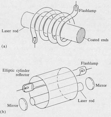
Figure 9.14. Typical designs for optically pumped solid-state lasers.

The Ruby Laser The rod of a ruby laser is made of synthetic sapphire (Al₂O₃), which is doped with approximately 0.05 percent by weight of Cr₂O₃. This concentration produces a pink-colored material. The color is due to the presence of Cr³⁺ ions, which replace aluminum in the crystal lattice.

An energy-level diagram of Cr³⁺ in ruby is shown in Figure 8.17 of the previous chapter. In operation of the laser the pumping light is absorbed by the Cr³⁺ ions raising them from the ground state ⁴A to either of the excited states ⁴T₁ or ⁴T₂. From these levels a rapid radiationless transition to the level ²E takes place. Decay from ²E is relatively slow, so that with sufficient excitation a population inversion between ²E and the ground state ⁴A can occur. When this condition attains, amplification occurs at the wavelength 6934 A, corresponding to the transition ²E → ⁴A. The resultant output is an intense pulse of light at this wavelength.

Other Solid-State Laser Materials Besides ruby, a number of other crystals, when doped with impurity atoms containing incomplete subshells, have been found to exhibit stimulated emission. Neodymium, for example, has a laser transition at about 1.06 μ. Various host solids have been used with neodymium, including crystals of calcium fluoride (CaF₂) and calcium tungstate (CaWO₄), as well as glass. Neodymium-doped yttrium aluminum garnet (YAG) has proved to be very efficient as a lasing crystal. YAG lasers can be operated continuously when pumped with incandescent tungsten lamps. Table 9.2 lists a number of examples of solid-state laser materials.

Table 9.2. SOME SOLID-STATE LASERS

9.9 Dye Lasers

Stimulated emission in liquid solutions of fluorescent organic dyes was first reported in 1966 by Sorokin and Lankard at the IBM laboratories. The dye solutions were optically pumped with a ruby laser, and in later experiments with a fast flash lamp. In the organic dyes used in lasers, such as fluorescein and rhodamine, the fluorescence bands are quite broad, typically 50 to 100 nm. The amplification bands are correspondingly broad, and it is thus possible to vary the output frequency of the laser by the use of tuning elements (prisms, gratings, and interferometers) inserted in the laser cavity.

Previous to the advent of the dye laser, only a finite number of discrete laser frequencies was available. Now, with a wide selection of lasing dyes, the entire region of the optical spectrum from the near ultraviolet to the near infrared can be spanned. Continuous-wave operation of the dye laser has been achieved by using a continuous-wave gas laser (argon or krypton) as the optical pump source. A diagram of a typical continuous-wave tunable dye laser is shown in Figure 9.15. Table 9.3 lists the tuning ranges of some laser dyes.

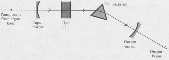
Figure 9.15. A tunable dye laser arrangement. The input mirror is transparent to the argon laser pump beam, but is highly reflecting over the tuning range of the dye.

Table 9.3. SOME LASER DYES

Dye	Approximate Tuning Range (nm)
Cresyl violet	640—700
Rhodamine B	580—690
Acridine red	600—630
Rhodamine 6G	560—650
Sodium fluorescein	520—570
4 Methylumberiferone	440—540
Coumarin	440—490
Diphenyl anthracene	430—450
Sodium salicylate	390—420
POPOP	380—440

9.10 Semiconductor Diode Lasers

The most compact laser is the semiconductor diode laser, also called the injection laser. In its simplest form the diode laser consists of a p-n junction in a doped single crystal of a suitable semiconductor, such as gallium arsenide. When a forward bias is applied to the diode, electrons are injected into the p side of the junction and holes are injected into the n side. The recombination of holes and electrons within the junction region results in recombination radiation. This is the principle for the operation of light-emitting-diode (LED) devices that are used for many applications—such as numerical display in electronic computers—in which spontaneous recombination radiation is produced. If the junction current density is large enough, a population inversion can be obtained between the electron levels and the hole levels. Stimulated emission can then occur and laser action commences when the optical gain exceeds the loss in the junction layer. In diode lasers this layer is thin, typically of the order of a few microns, and the end faces of the crystal are made partially reflective to form an optical resonator. The threshold current density for gallium arsenide injection lasers is about 10⁴ A/cm², and the emitted radiation is in the near infrared, about 830 to 850 nm.

9.11 Q-Switching and Mode Locking

In high-power lasers that are pumped by intense optical pulses the lasing action begins when the population-inversion density reaches a certain threshold value, namely, when the optical gain exceeds the loss. The reciprocal of the fractional loss per cycle is known as the resonant Q of the cavity. The lower the loss, the higher the Q and the lower the inversion density required for oscillation, and conversely. In high-power pulsed lasers the inversion density is quickly “used up” as soon as laser oscillation commences. By delaying the onset of oscillation it is possible to obtain a higher inversion and thus higher output than would otherwise be obtained. This is achieved by inserting a suitable optical shutter, known as a Q switch, into the laser cavity. The shutter is closed at the beginning of the pump pulse and opened when the population inversion is maximum.

There are various methods of Q switching. A simple method is to rotate one of the resonator mirrors at a high rate about an axis perpendicular to the optical axis of the laser cavity. This “spoils” the cavity and prevents oscillation except for a very brief time during the rotation cycle. A second method makes use of an electro-optic shutter in the laser cavity. Pockels cells are commonly used for this application. The Pockels cell is “opened up” with a high-voltage pulse that is appropriately delayed relative to the optical pump pulse. A third method employs what is known as a saturable absorber. This is a certain type of dye which bleaches out or becomes transparent when strongly irradiated so that the upper levels are saturated and thus no more absorption can occur. This is known as passive Q switching.

By the use of Q switching it is possible to attain very high peak powers. Pulses in the 100-MW range are common with ruby and neodymium-glass lasers. Also, the pulse duration is shortened from typical values of a few microseconds for conventional operation to a few nanoseconds for Q-switched operation. Even higher powers can be attained by passing the output beam of a Q-switched laser through an amplifier or a series of amplifiers. In this way it has been possible to produce pulses in the gigawatt (GW) and terawatt (TW) region. These extremely high powers are necessary for laser fusion.

Mode Locking If a nonlinear absorber, such as a bleachable dye, is placed in the resonator cavity of a laser, it is often found that the laser output is changed into very short, regularly spaced pulses. The time separation between successive pulses is found to be the round-trip time for light in the optical cavity (or sometimes a simple fraction, , ... of the round-trip time). Thus the radiation inside the cavity has become “bunched” into one or more narrow pulses that bounce back and forth between the resonator mirrors. Now a simple Fourier analysis shows that the frequency spectrum of a regular pulse train consists of a number of discrete frequencies separated by the repetition frequency of the pulses. Since the round-trip time is 2d/u, where d is the mirror spacing and u is the velocity, then the frequency spectrum of the pulse train consists of components separated by the longitudinal mode spacing ul2d (or an integral multiple of it). However, unlike a conventional laser that is oscillating on several different longitudinal modes simultaneously but in a mutually incoherent phase relationship, the phases in the case of regular pulsing are necessarily related in a definite way. Hence the pulsing laser is said to be mode locked or phase locked.

Now the width of a single pulse is equal to the reciprocal of the total frequency bandwidth involved, according to the discussion of Section 4.6, Equation (4.33). For a mode-locked laser this is the total bandwidth occupied by the oscillating modes. Hence if there are N such modes, the temporal width of each pulse is the fraction 1/N of the time interval between successive pulses. Thus lasers having a broad frequency band of amplification can support a large number of modes and are therefore capable of producing very short mode-locked pulses.

In the case of gas lasers, such as the helium—neon or the argon laser, which oscillate on a narrow atomic line transition, the mode-locked pulses are limited in narrowness to about a few nanoseconds. On the other hand, with dye lasers and the neodymium-glass laser that have broadband capability, mode-locked pulses in the picosecond range are produced.

It is interesting to note that a 3-ps pulse measures only about 1 mm thick, as a typical example. The radiation in such cases can truly be said to be concentrated into a thin “sheet” that travels with the speed of light.

9.12 The Ring Laser

The ring laser is an example of a technological application of lasers. It is a device designed to measure rotation by means of counterrotating coherent light beams and was developed in 1963 at the Sperry-Rand Corporation. The device is the laser analogue of the Sagnac experiment (Section 1.4 in the Appendix).

The basic design is shown in Figure 9.16. The optical cavity of the laser consists of four mirrors arranged in a square. One or more laser tubes are inserted into the cavity to provide amplification. Oscillation occurs at those resonance frequencies

which lie within the amplification curve of the laser medium. Here L is the effective length of the complete loop and n is an integer.

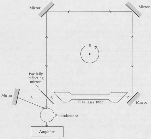
Figure 9.16. The ring laser.

If the system is rotating about an axis perpendicular to the plane of the loop, the effective path lengths for the clockwise and the counterclockwise beams are different. This results in a difference ∆v between the frequencies of the laser oscillation of the two beams. The difference is

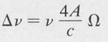
where v is the frequency of the laser when it is not rotating, A is the loop area, and Ω is the angular speed of rotation.

In the operation of the ring laser, the method of optical heterodyning is used. The two output beams of the laser are brought together and fed to a photodetector as shown. The output of the photodetector consists of a beat signal whose frequency is equal to the difference ∆v. This, in turn, is proportional to the angular speed of rotation.

PROBLEMS

• 9.1 The first line of the principal series of sodium is the D line at 590 nm. This corresponds to a transition from the first excited state (3p) to the ground state (3s). What is the energy in electron volts of the first excited state?
• 9.2 What fraction of sodium atoms are in the first excited state in a sodium vapor lamp at a temperature of 250°C?
• 9.3 What is the ratio of stimulated emission to spontaneous emission at a temperature of 250°C for the sodium D line?
• 9.4 Calculate the gain constant of a hypothetical laser having the following parameters: inversions density = 10¹⁷/cm³, wavelength = 700 nm, line width = 1 nm, spontaneous emission lifetime = 10^-4 s.
• 9.5 Calculate the inversion density N₂–N₁ (g₂/g₁) for a helium-neon laser operating at 633 nm. The gain constant is 2 percent /m, and the temperature of the discharge is 100°C. The lifetime of the upper state against spontaneous emission to the lower state is 10^-7 s.
• 9.6 If the spot size at the mirrors of a helium—neon laser is 0.5 mm, what is the length of the laser cavity? The cavity is of the confocal-type, and the wavelength is 633 nm. What is the spot size of the 3.39-μm transition in the same cavity?
• 9.7 Limiting apertures are placed at the mirrors of a confocal cavity in order to suppress the higher modes. If the cavity is 1 m in length, what should the diameter of the apertures be in order that the loss for the TEM 0,1 mode be 1 percent? What is the corresponding loss for the TEM 0,0 mode? (See Figure 9.10.) The wavelength is 633 nm.
• 9.8 Prove Equation (9.30) giving the difference frequency of the ring laser.