The trees of the mid-twentieth century, especially those of scientists such as Alfred Sherwood Romer and George Gaylord Simpson, emphasized the grand unfolding radiations of life over geologic time, very much in accord with perceptions of a Darwinian view of evolution. By the 1970s, perceptions and research programs, including how to build and show trees, began to change radically for three reasons. First, in the 1960s two new, quite different schools of biological systematics emerged that challenged how one assesses relationships and how one represents these relationships visually. Second, although biochemically and genomically based phylogenetic studies began before the invention of the polymerase chain reaction (PCR) procedure in 1983, this invention was a watershed that made the analysis of vast quantities of genetic information possible. In addition, an apparent threat to tree iconography emerged as molecular studies expanded. Simple organisms possess fewer anatomical characters than more complex organisms that might be useful in systematics studies, and these simpler organisms also left less of a fossil record. More powerful molecular tools permitted a more thorough comparison of these simpler organisms, but they also threatened the very tree iconography by arguing instead that life’s history represented an interwoven web or Darwinian tangled bank. Third, computing power increased by leaps and bounds in the latter half of the twentieth century, making the analysis of vast data sets possible. These three changes affected how we perceive evolution, how we show this on trees and other sorts of diagrams, and even how we ourselves, within this scheme, changed forever—all of which made for a true scientific and technical revolution.
Three Schools
No matter how one wishes to define it, much of the study of evolution is as a historical science. The origin of life on planet Earth happened once, or once at least as we suspect. At any rate, this was a singular event or maybe a series of events in which we have participated and which we have observed. This means that uncovering the process and pattern of what until at least recently entailed a paleontological and anatomical approach lay outside of what was regarded as scientifically testable. Even giants of evolutionary tree construction such as Ernst Haeckel, William King Gregory, Romer, and Simpson in the end used their superior knowledge of the subject to argue that this or that tree was likely correct. This science done by appeal to authority became known as “evolutionary systematics” compared with the newly arising and arguably more testable schools of “numerical taxonomy” and “phylogenetic systematics”
Beginning in the 1960s, this appeal to authority began to wane, and no less an authority than Simpson realized this shift in ideas. In Principles of Animal Taxonomy (1961), he writes, “I shall here acknowledge a debt to Hennig (1950), which is certainly one of the most valuable books on taxonomy…that has yet appeared,” but he notes that his agreement with Hennig’s approach may be “only partial, but it is substantial” (71n.2). He was referring to Willi Hennig’s (1913–1976) then obscure and difficult book Grundzüge einer Theorie der phylogenetischen Systematik (Outlines of a Theory of Phylogenetic Systematics, 1950), about which the great evolutionist Ernst Mayr (1982) noted that it “is written in rather difficult German, some sentences being virtually unintelligible” (226), a rather damning statement from a German-born and German-educated American biologist. Mayr was not alone in his assessment of the book. Additionally, Hennig did not seem to know or at least did not cite much of the work of other great systematists of the time; nevertheless, Simpson must be given credit for his prescient take on the significance of Hennig’s work. In his autobiography, Simpson (1978) expounded less kindly about Hennig’s ideas, likely because by then the Hennigian school of systematics had continued its ascendency and with it various methods of visualizing evolutionary relationships. Much of this eventual success can be attributed to the translation, clarification, and rewriting of Hennig by Dwight Davis and Rainer Zangerl in Phylogenetic Systematics (1966), also the eponym of the Hennigian school. Even with Simpson’s (1961) laudatory comments, Hennig’s ideas were known best to German-speaking entomologists until the largely rewritten English version of his book.
The impact of Hennig on our perceptions of how evolution occurred and how best to analyze and represent it cannot be overemphasized, and yet as is often the case, the current state of the sciences traverses far beyond what Hennig might have imagined. As noted at its Web site, “the Hennig Society was founded in 1980 with the expressed purpose of promoting the field of Phylogenetic Systematics. Hennig’s idea that groups of organisms, or taxa, should be recognized and formally named only in cases where they are evolutionarily real entities, that is ‘monophyletic,’ at first was controversial. It is now the prevailing approach to modern systematics.” Just how profoundly Hennig’s German-language book (1950) differs from the English-language book (1966) becomes clear in what he chose to illustrate. The 370-page book from 1950 has fifty-eight figures dominated by twenty maps with biogeographic distributions mostly of insects and eleven illustrations of insect anatomy, whereas only ten present one or more tree-like diagrams of some sort. By contrast, the 263-page book from 1966 has sixty-nine figures of which only seven show maps and six show anatomy, whereas forty-five present one or more tree-like diagrams. As with Darwin a century before, Hennig realized that a major key to the understanding of evolutionary history is a good knowledge of the biogeographic distributions of species. Clearly, a profound change occurred in the sixteen years between the publication of the original and the translated text, but Hennig did not diminish the role of biogeography. Rather, he expanded and developed how to probe for the underlying methodology for building and drawing tree-like diagrams. These became commonly known as cladograms by virtue of the clades, or branches (Gk. kladoi), that form the diagram and thus provided the simplified name for this school of systematics: cladistics.
Stated simply, cladistics tries to tease apart the similarities or characters that species and higher taxa share by virtue of a common ancestor versus those they retain from a common ancestor or those that arose through similar ecological constraints. Figure 7.1A, found in Phylogenetic Systematics (1966) but not in Grundzüge (1950), shows the development of Hennig’s ideas related to this topic. For the uninitiated, the use of lowercase and uppercase letters in figure 7.1A at first might be confusing. The common ancestor of A, B, and C, which is unlabeled, possessed characters a, b, and c. Character a was transformed to a' only in taxon C so is unique to C. The ancestral character was retained in A and B, and thus is a shared-ancestral character, or a symplesiomorphy in Hennig’s terminology, but being ancestral, such retentions are not useful in arguing evolutionary relationships between such taxa as A and B. Character b was transformed to b' in the unnamed common ancestor of B and C, and thus is a shared-derived character of B and C, or a synapomorphy in Hennig’s terminology. This makes it useful in arguing that B and C share a more recent ancestor with each other than either does with A. Finally, c was transformed to c' separately in both A and C, likely as the result of similar ecological constraints, and thus they are the result of convergences. Synapomorphies and symplesiomorphies collectively represent homologies or similarities resulting from a common descent, more recent for synapomorphies and farther in the past for symplesiomorphies. Convergences caused by similar ecological constraints are often called homoplasies in juxtaposition to homologies. To establish a reasonable hypothesis of evolutionary relationships, in most real cases we need to evaluate many more than the three characters shown in Hennig’s hypothetical case.
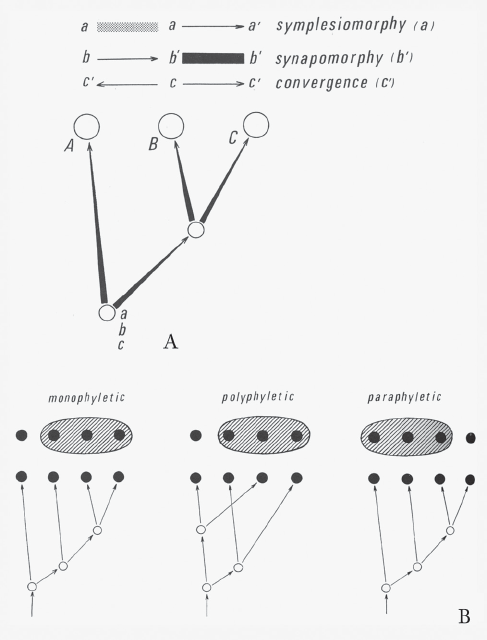

FIGURE 7.1 Willi Hennig’s diagrams of the concepts of (A) symplesiomorphy, synapomorphy, and convergences, and (B) monophyly, polyphyly, and paraphyly, from Phylogenetic Systematics (1966). (Reproduced with permission of the University of Illinois Press)
A simple example may suffice. Birds possess wings because their most recent common ancestor evolved wings; thus wings in birds are a synapomorphy for birds relative to other nonflighted vertebrates, but wings cannot be used to argue relationships among birds because they are a symplesiomorphy within Aves (birds). In contrast, the presence of wings in birds, bats, and insects occurs not because of common descent but because of the ecological constraint of the need for wings for flight—that is, a convergence (or homoplasy). Each of these three groups evolved wings from a separate ancestry, which is quite clear in this case because the underlying structures of the wings are so profoundly different. Synapmorphies form the basis for building cladograms because they arise from common descent. Hennig began developing these ideas in Grundzüge (1950), with a much clearer explanation in Phylogenetic Systematics (1966). One might ask why these ideas that appear deceptively simple were not codified earlier. In fact, a number of biologists presaged Hennig’s ideas, but it was Henning and especially some of his early followers who rather strictly tried to follow the dictum that a cladogram must be built using only synapomorphies arising from the common ancestry of a given group, or, more correctly, the common ancestry for a clade. Hennig and his adherents argued further that any resulting classification must adhere to the underlying cladistic analysis. Another diagram found in Phylogenetic Systematics but not in the earlier Grundzüge shows the basis for this classification (see figure 7.1B). As Hennig labels them for the diagram, groups are monophyletic if they are based on synapomorphies, paraphyletic if based on symplesiomorphies, and polyphyletic if based on convergences.
It was and still is the issue of classification and not the philosophy of the cladistic analysis that caused the greatest consternation for biologists. Biologists can be quite conservative, not easily giving up older ways of doing things, such as the Linnaean system. An organization somewhat more sympathetic to a Hennigian classificatory system, the International Society for Phylogenetic Nomenclature, advocates the development of a classification called the Phylocode that someday may replace or at least supplement the Linnaean system. The issues become quite clear with a classic example of how to classify tetrapods, which traditionally include Amphibia, Reptilia, Aves, and Mammalia. Although the placement of Testudines (turtles) remains in flux, the three identical cladograms in figure 7.2 show the traditional view of tetrapod relationships. Using Hennigian principles, one can ask what synapomorphies traditional reptiles share. Certainly they have scales, but so do a number of mammals on their tails and birds on their legs. Feathers are, in fact, modified scales. Reptiles also share cold-bloodedness and, except for crocodilians, possess a three-chambered heart. These, however, are symplesiomorphies for Reptilia or synapomorphies of a much earlier ancestor and thus tell us nothing about relationships within Reptilia. A cladistic classification includes Aves within Reptilia, making it monophyletic, or what Hennig designated as holophyletic. This was and to a lesser extent remains anathema to some biologists. A monophyletic group or a clade (see figure 7.2A) includes the most recent common ancestor (the asterisk in figure 7.2A–C) and all its known descendants. The more traditional grouping of Reptilia forms a paraphyletic group (see figure 7.2B) because it excludes one descendant clade (Aves), although the most recent common ancestor is included. Some biologists argue that both monophyletic and paraphyletic groups should be recognized, but at most no one argues that the third kind, called a polyphyletic group, should be recognized. In the example in figure 7.2C, Haemothermia, meaning “warm-blooded,” was proposed by Richard Owen in the nineteenth century and revived for a short time in the 1980s (Gardiner 1982). Such polyphyletic groups have neither all known descendants nor the most recent common ancestor.

FIGURE 7.2 An example within Vertebrata showing (A) monophyletic Reptilia, (B) paraphyletic Reptilia, and (C) polyphyletic Haemothermia. (Adapted from various sources)
Between Hennig’s Grundzüge (1950) and Phylogenetic Systematics (1966), we see how other of his ideas and visualizations of these ideas transformed. Like his countryman Haeckel, Hennig utilized a variety of terms and representations. The relationship between ontogeny and phylogeny, terms that Haeckel coined, interested both men. In Grundzüge, Hennig shows us a relatively simple rendition based on earlier sources of what he terms the tokogenetic relationships—that is, genetic relationships between individuals in a species (read left to right), specifically females and males represented as empty and filled circles, respectively (figure 7.3A). Although representing a sexually reproducing species, the connecting lines do not present a clear delineation of reproduction and descent. This becomes far more explicit and clearer in Phylogenetic Systematics, in which Hennig presents three figures, each more complex than that in Grundzüge, explaining tokogenetic relationships. Each succeeding diagram adds additional complexity, with that shown in figure 7.3B the most complex, combining Hennig’s ideas of genetic relationships of individuals in sexually reproducing species with his ideas of transformations within the ontogeny of an individual and the process of speciation. As an entomologist, Hennig concerned himself more than other biologists might with the radical morphological changes undergone by some insects from larva to pupa to adult. He called each of these stages a semaphoront in the metamorphosis during the ontogeny of an individual, something of less obvious concern to, for example, an ornithologist studying birds. These semaphoronts then combined to form the ontogeny of a male or female, which, in turn, would mate to form the next individual. In combinations, these repeated life cycles, matings, and life cycles formed what Hennig termed cyclomorphism. If a barrier to breeding should form (the wedge in figure 7.3B), populations could split, establishing separate breeding populations and ultimately forming two or more new species. Hennig combined all these ideas in what he called hologenetic relationships, or what we today usually refer to as monophyly, discussed previously, in which one or more species can be traced to a common ancestry. Hennig provides us with a small, coarser-scaled diagram to the right emphasizing the next higher level in these ongoing ontogenetic and phylogenetic processes. His ideas on recovering monophyletic relationships endure in modern systematics, whereas much of his nomenclature of these processes does not.
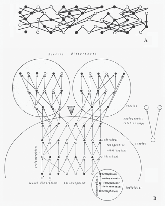
FIGURE 7.3 Hennig’s (A) relatively simple depiction of the tokogenetic, or genetic, relationships between individuals in a species, specifically females and males, redrawn from Grundzüge einer Theorie der phylogenetischen Systematik (1950), and (B) more explicit and clearer figure showing tokogenetic relationships, combining his ideas of genetic relationships of individuals in sexually reproducing species with his ideas of transformations within the ontogeny of an individual (semaphoronts) and the process of speciation (wedge), from Phylogenetic Systematics (1966). ([B] reproduced with permission of the University of Illinois Press)
When Hennig began his endeavors, computing was in its infancy and thus earlier attempts at cladistic reconstructions were done by hand. The methods of representation varied, but often the sort of horizontal bars shown in figure 7.4A were drawn across a cladogram to show how characters transformed along the various clades. Such representations became scarcer as computing power increased and the number of characters to be analyzed rapidly expanded. The Swedish entomologist Lars Brundin (1897–1993) was one of the earliest and most influential advocates for Hennig’s ideas. In 1965 (and in a longer paper in 1966), Brundin proved to be an even better spokesman for Hennig’s methodology with the publication of “On the Real Nature of Transantarctic Relationships,” in which he examined the phylogenetic relationships and biogeography of one group of chironomid midges. Except for entomologists, few students of evolution knew of chironomid midges, other than possibly field scientists who understood these flies to be pesky but thankfully nonbiting. Brundin provided one of the first studies in English demonstrating Hennig’s methodology for not only the phylogenetic reconstruction of a specific group but also its biogeographic history using similar techniques. Brundin’s cladogram follows Hennig’s ideas and uses similar iconography, showing plesiomorphies as open rectangles, symplesiomorphies as open rectangles joined by a thin line, apomorphies as solid rectangles, and synapomorphies as solid rectangles joined by gray bars (see figure 7.4A). The horizontal arrows refer to specific character transformations, such as characters 38 and 39 (near the middle of the cladogram) transforming from the plesiomorphic (ancestral) states in the clade on the left to the apomorphic (derived) states in the clade on the right. The transformation of character 40 occurred in the opposite direction. Lower on the diagram, Brundin shows us where in the cladogram his analysis suggests these evolutionary transformations took place. This profoundly new and different approach that Hennig advocated and that Brundin so aptly demonstrated offered a hypothesis of relationships that could be explicitly tested. Nothing quite like it had come before. With this testable hypothesis of relationships, Brundin further demonstrated what Hennig also advocated: that such hypotheses of relationship could also provide a hypothesis of relatively when and how these various clades reached their present biogeographic ranges in what became known as area cladograms (see figure 7.4B). It must be kept in mind that both the cladogram of relationships and that of biogeographic history are hypotheses, but as we see, neither had been so explicitly and scientifically (testably) expressed before.

FIGURE 7.4 Lars Brundin’s (A) cladogram and (B) area cladogram for chironomid midges, from “On the Real Nature of Transantarctic Relationships” (1965). The cladogram shows the method of representation developed by Hennig. (Reproduced with permission of the Society for the Study of Evolution)
The second new school of “numerical taxonomy” as developed mostly through the efforts of the biologists Peter Sneath (1923–2011) and Robert Sokal (1926–2012) briefly remained at the fore for a relatively short time, basically in the 1960s and 1970s. In their two major works, Principles of Numerical Taxonomy (Sokal and Sneath 1963) and Numerical Taxonomy (Sneath and Sokal 1973), they argued that biological classifications should be based on overall similarities of species rather than on assumptions about unknowable evolutionary relationships, although they granted that when done properly, the classification to some extent reflected evolutionary history. In their earlier book, Sokal and Sneath (1963) write: “In developing the principles of numerical taxonomy, we have stressed repeatedly that phylogenetic considerations can have no part in taxonomy and in the classificatory process. Once a classification has been established, however, biologists will inevitably attempt to arrive at phylogenetic deductions from the evidence at hand” (216).
Sneath and Sokal’s (1973) discussion of a figure contrasts clearly the distinction between numerical taxonomy and phylogenetic systematics (figure 7.5A). In this hypothetical phylogenetic tree, lineage x departs phenetically, or in its overall similarity, from its nearest relatives in cluster A that resemble more members of cluster B. About this the authors write, “Although the divergence of x from cluster A is of great evolutionary interest, the overall similarity of x to the members of cluster B is more useful” (57), but this prompts the question as to what “useful” refers. These views were anathema to cladists, for whom the main objective or “usefulness” of a classificatory scheme was to reflect evolutionary history as nearly as possible. For them, a hypothesis of evolutionary history based on a phylogenetic analysis came before attempts at classification. Cladists’ establishment of this objective occurred, as discussed earlier, by grouping taxa based on shared-derived characters or synapomorphies, which arguably reflected evolutionary history.

FIGURE 7.5 Peter Sneath and Robert Sokal’s (A) hypothetical phylogenetic tree showing lineage x, which they would classify with cluster B rather than cluster A because of phenetic similarities to B; (B) rooted phenogram with OTU numbers on the right and frequency distributions of similarity coefficients along the horizontal axis; and (C) phenogram translated into a taxonomy using percentage-based phenons, redrawn from Numerical Taxonomy (1973).
In numerical taxonomy, analyses of overall or phenetic traits of organisms increasingly were based on the then newly emerging computer-based algorithms from which one could obtain an arguably objective taxonomy. In addition to an increased reliance on computers, one very useful term that outlived phenetics is “operational taxonomic unit” (OTU), generally defined as “the taxonomic unit of sampling used by the researcher in a particular study.” OTUs may be individual organisms, populations, species, genera, and so forth, or, for microbiologists, strains of bacteria, which are not easily classified in traditional taxonomic schemes. The results of phenetic analyses sometimes appeared as unrooted networks with distances between the OTUs indicating the degree of overall similarity. Although no longer common in building higher-level phylogenetic studies, such networks remain an important tool in population studies within a species or even very closely related species because the goal is an assessment of intertwining genetic affinities rather than phylogenetic reconstruction per se.
Sneath and Sokal (1973) referred generally to tree diagrams as dendrograms, as had others, with the further distinction for cladograms constructed by phylogenetic systematists, whereas phenograms refer to dendrograms derived from phenetic analyses. Phenograms do not represent the hypothesis of descent from a common ancestor inherent in cladograms. When used, visual representations varied but most commonly appeared as rooted phenograms that opened up, down, or, in the common case, from left to right (see figure 7.5B). In this example from a source used by Sneath and Sokal (1973), the OTUs are the numbers on the right. The authors identify the numbers at the top and the horizontal lines with small hash marks within the figure as “frequency distributions of similarity coefficients”—in other words, as a measure of overall similarity rather than any argument for recency of common ancestry. Such analyses might or might not be the same as their evolutionary counterparts. When this phenetic information translates into a taxonomy, overall similarity arguably provides the best basis for classification. One possible way is to divide a phenogram into levels or percentages of overall similarity. OTUs of a given level or percentage of similarity could be thus grouped, such as the so-called percentage-based phenons (see figure 7.5C). This presents a good example of the push for objectivity leading instead to arbitrariness in taxonomic classification.
Although unquestionably accepting evolution, Sneath and Sokal argued that recovery of its history was difficult or impossible to accomplish. They claimed that when done properly, a phenetic classification to some extent reflected parts of evolutionary history. The question remains: What parts of evolutionary history are reflected under the aegis of phenetics? Even though phenograms and cladograms superficially resemble each other in being tree-like, just as with the nonevolutionary and evolutionary trees of the nineteenth century, the intentions of the two diverge quite markedly from each other. Once again, very similar iconography meant something quite different, depending on the underlying theoretical framework used to generate it. In the end, phylogenetic systematics/cladistics took hold while numerical taxonomy/phenetics faded, as measured by the number of books that the former school rather quickly spawned. Books espousing phylogenetic systematics/cladistics appeared soon after the reprinting in 1979 of Hennig’s Phylogenetic Systematics (1966) (for example, Eldredge and Cracraft 1980; Nelson and Platnick 1981; Wiley 1981), but not those promoting numerical taxonomy/phenetics following the publication of Sneath and Sokal’s Numerical Taxonomy (1973). The rise of both molecular tools and far more powerful computing certainly accelerated this shift, but, more important, an underlying desire drove it: the need to understand how species relate one to another and, most important, how humans relate to other species. Cladistics strove to provide the answer, whereas phenetics did not.
The Molecular Approach to Tree Building
At the same time as the schools of numerical taxonomy/phenetics and phylogenetic systematics/cladistics emerged with more objective methods of building trees and creating classifications, other new technologies further revolutionized the reconstruction of life’s history. These new, molecularly based technologies allowed us to explore in far greater detail and depth how cells function, how proteins are synthesized, and how genetic information is passed from one generation to the next. As with anatomical characters, molecularly based characters varied in what they represented. Recall that in the latter half of the nineteenth century, St. George Jackson Mivart (1865, 1867) used various aspects of primate postcranial anatomy to explore primate relationships, knowing full well that these characters alone could not provide a complete portrait of primate evolution. In the mid-twentieth century, William King Gregory had taken this approach to a greater and more integrated scale in the study of various organ systems and how they integrate to form the whole—an advance that proved very useful in phylogenetic reconstruction. So, too, when molecularly based analyses became possible, they began by using more clearly expressed cellular-level functions and those that could relatively easily be analyzed across various species. Thus the earliest attempts at molecular systematics did not look directly at the basis of genetics—deoxyribonucleic acid (DNA) and ribonucleic acid (RNA)—but indirectly at the products of these molecules: proteins and their building blocks, amino acids. Other early attempts were even more indirect, using the strength of immunological responses to infer closeness of relationship. In these early stages of molecular systematics, little concern arose as to which school of systematics should be used, although most would fall within the purview of phenetics because they examined overall similarity.
Tree-like diagrams using molecular or genetic data began to appear in earnest in the early 1960s, some ten years after the discovery and description of DNA in the early 1950s. The truly embryonic stages of molecularly based analyses, quite surprisingly, occurred far earlier than usually recognized, with the first attempts at molecular systematics dating to the very beginning of the twentieth century (Wood 2012). In 1901, the American British bacteriologist George H. F. Nuttall (1862–1937) reported comparing upward of 230 blood samples for all classes of vertebrates. In 1902, the work of British physiologist Albert S. F. Grünbaum (1869–1921, name changed to Leyton in 1915) with blood serums showed the great similarity among humans, chimpanzees, gorillas, and orangutans, arguably making him the pioneer of comparative primate serology (Wood 2012). Nuttall wrote additional papers on the topic with other colleagues, producing in 1904 an impressive 444-page monograph in which he demonstrates “certain blood-relationships amongst animals as indicated by 16,000 tests made by myself with precipitating antisera upon 900 specimens of blood obtained from various sources” (vii). In this monograph, Nuttall did not provide a phylogenetic tree based on his results, but he did include a tree about which he notes: “According to Dubois (1896) the relationships amongst the Anthropoidea are represented by the accompanying genealogical tree, based upon that of Haeckel (1895)” (figure 7.6A). He goes on to describe Eugène Dubois’s ideas on the fossil species included on the diagram, following which he continues, “the fact remains, that the degrees of reaction obtained by me in my blood tests are in strict accord with this genealogy, as pointing to the more remote relationship of the Cercopithecidae, but especially of the New World monkeys” (2). The relationships as shown do not differ greatly from those presented some sixty years later and accepted today, except that now chimpanzees (“Anthropopithecus”) are grouped with humans rather than with gorillas, a change not suggested until the early 1960s.

FIGURE 7.6 (A) Phylogenetic tree, modified after one in Eugène Dubois’s “Pithecanthropus erectus, eine Stammform des Menschen” (1896), showing relationships among Anthropoidea that agree with the results from George Nuttall’s blood serum results, from Blood Immunity and Blood Relationship (1904); (B) Vincent Sarich and Allan Wilson’s tree for primate evolution, showing an unresolved tripartite relationship among humans, chimps, and gorillas with a quite recent timing for this split, from “Immunological Time Scale for Hominid Evolution” (1967); Emile Zuckerkandl and Linus Pauling’s downward-opening trees, showing (C) the process of gene duplication and (D) the evolutionary relationships of some mammalian hemoglobin chains relative to the species in which they occur, modified from “Evolutionary Divergence and Convergence in Proteins” (1965). ([B] Reproduced with permission of the American Association for the Advancement of Science)
The early 1960s proved pivotal in the publication of papers using molecular techniques to produce phylogenies; some were more theoretical, whereas others presented specific results. In 1965, the supposedly first phylogeny using the principle of parsimony was published by Luigi Cavalli-Sforza and Anthony Edwards, showing relationships of humans populations based on blood-group polymorphism gene frequencies (Pietsch 2012)—that is, the relative frequencies of the blood types A, B, AB, and O in human populations. In 1964, a paper written in English by Emile Zuckerkandl (1922–2013) and Linus Pauling (1901–1994) was translated and published in Russian; in 1965, it was published in English with the intriguing title “Molecules as Documents of Evolutionary History.” Although the paper lacks a tree figure, Zuckerkandl and Pauling (1965b) noted in the very first sentence of the abstract: “Different types of molecules are discussed in relation to their fitness for providing the basis for a molecular phylogeny.” They continued that “semantides,” a term they coined for “the different types of macromolecules that carry the genetic information or a very extensive translation thereof” (rRNA, rDNA, and so on), would work best for such research (357).
In a book chapter, Zuckerkandl and Pauling (1965a) discussed the evolution of proteins, notably of the mammalian hemoglobin chains—that is, variations in the subunits of hemoglobin, the protein that transports oxygen in the red blood cells of vertebrates. The paper includes two downward-opening diagrams, the first of which deals with the process of gene duplication yielding what they called β (beta), γ (gamma), and δ (delta) chains of hemoglobin, clearly providing a phylogeny of this protein rather than of any organisms (see figure 7.6C). The second figure, also downward opening, at first appears to show a phylogeny of humans, horses, and cattle using the same protein (see figure 7.6D). It would be an odd phylogeny indeed that has horses sharing a closer ancestry with some humans than these humans share with other humans—shades of the centaur? It becomes clear in both the labeling of the diagram and the discussion that this study analyzes the probable evolutionary changes of some mammalian hemoglobin chains rather than the relationships of the species in which these hemoglobin chains occur. Nonetheless, Zuckerkandl and Pauling note that results such as these offer an intriguing possibility for doing phylogenetic studies but that the evidence alone cannot be taken seriously, as it relies on a single protein—again shades of Mivart’s late-nineteenth-century caution about using single organ systems to deduce relationships. How gene families evolve remains a rich area of study along with the potentially vexing issue of how to relate gene trees with the evolutionary history of the organisms that contain them, inasmuch as the two sometimes are not congruous. These results offer an early warning that the evolutionary history of molecules does not always neatly track one for one the history of the species in which they occur.
In the same chapter, Zuckerkandl and Pauling (1965a) described a hypothesis that they had been promoting for the previous three years, which they called the molecular evolutionary clock (Morgan 1998). In one form, the hypothesis argues that the amino acids composing a given protein (or other noncoding parts of the genome), not being under selective pressure, change in a stochastically constant manner over time, thus approximating clock-like change. In theory, then, this “clock” can be used to estimate the time since two given species or other groups split one from the other; fossils need not apply to establish this event, but as we shall see, this has become a major area of contention between molecularly based and anatomically based systematists concerning the timing of some major evolutionary events. Although Zuckerkandl and Pauling’s chapter helped set the stage for what followed, its most frequent citation comes not because of the early molecular trees discussed earlier but for the molecular clock hypothesis.
A second molecular technique championed in the 1960s in the laboratory of Allan C. Wilson (1934–1991) became known as the microcomplement fixation method. The technique relied on the fact that an organism’s body builds antibodies in an immunological response to foreign substances termed antigens—in this case, between various proteins. The closer two species relate to each other, the stronger the antigen–antibody response, such as between a chimpanzee and a human versus either of these species and a species of baboon. Assumptions for this analysis rely on the hypotheses that the differences seen between species relate to the amount of changes in amino acids within the proteins and, more controversially, that these changes follow some sort of molecular clock model such as that advocated by Zuckerkandl and Pauling (1965a, 1965b). Also, the technique measures overall similarity such as that advocated by numerical taxonomy.
Beginning in the 1960s, trees using this technique appeared, notably in a paper published in 1967 by Vincent Sarich (1934–2012) and Wilson, the mentor for his doctoral degree, dealing with primate evolution (see figure 7.6B). Showing an unresolved tripartite relationship among humans, chimps, and gorillas caused some controversy, but the quite recent timing of the split created a much greater yelp from critics. Sarich and Wilson arrived at a date of about 5 million years ago for this three-way split based on immunological distances, contrasting greatly with estimates of up to 30 million years based mostly on the fossil record. Current estimates based on fossils and molecules bracket this possibly complex speciation process between chimps and humans from 10 to 5 million years ago. More to the point, whereas Zuckerkandl and Pauling’s (1965a, 1965b) papers created smoke over the issue of a molecular clock, Sarich and Wilson’s (1967) paper set the place ablaze. Although both sides have given some ground—there is not one but many molecular clocks, and molecular methods sometimes resolve relationships not possible using fossils—the greatest issue remains the quandary over the timing of phylogenetic events and whether fossils, molecules, or both best address and answer these questions.
A paper by Morris Goodman (1925–2010) appears to predate Sarich and Wilson (1967) in arguing for the tripartite relationship among humans, chimps, and gorillas. Although not as explicitly, Goodman also suggested that some molecular changes are neutral relative to natural selection and hence could change in a stochastically random fashion. In 1963, Goodman published what he called a primate “classification from serological reactions” (that is, antigen–antibody reactions between blood serums of various mammalian species), although in the text he does refer to it as a dendrogram (figure 7.7A). While a classification is certainly part of this figure, it equally shows Goodman’s ideas of relationships among various primates, with other mammals as outliers. Particularly interesting, Goodman shows gorillas, chimpanzees, and humans as an unresolved tritomy, or three-way split, as Sarich and Wilson would do four years later. Further, Goodman rather audaciously places all three into the “human family,” Hominidae. Recall that although earlier workers well back into the nineteenth century, Darwin among them, argued for a special relationship between apes and humans, they never suggested placing them in the same family. Even in the middle of the twentieth century, to distinguish a special relationship among gorillas, chimpanzees, and humans to the exclusion of other apes was going too far for many, if not most, biologists. But unlike in preceding centuries, this had less to do with any obeisance to an Abrahamic God than with the quite obvious physical, behavioral, and intellectual differences separating humans from apes.
One person in particular at the meeting in 1962 at which Goodman presented his ideas of grouping gorillas, chimpanzees, and humans within Hominidae was George Gaylord Simpson (1963), who presented a paper for the volume in which Goodman’s paper also appeared (Washburn 1963). In his accompanying phylogeny, Simpson shows the traditional phylogenetic tree placing humans (Homo) to the right as quite distinct from the apes shown to the left (see figure 7.7B). Notably, Simpson includes chimpanzees and gorillas in his genus Pan. His classification later in the paper has only Homo and Australopithecus in Hominidae, with all but a few odd fossils placed in the ape family Pongidae. Simpson was not simply being obstreperous; recall that he, as did most supporters of the Modern Synthesis in the mid-twentieth century, championed Darwin’s adaptational changes and wished to reflect them not only in phylogenies but in classifications as well. Figure 7.7C clearly presents Simpson’s (1963) arguments that humans represent such a different ecological milieu from apes that they must be placed in a different “hominid zone.” As in figure 7.7B, Pan includes both gorillas and chimpanzees. Once again, Simpson is using a tree to argue his case not only for the pattern of evolution but also for its process. For Simpson, adaptational regimes play an important role in phylogenetic reconstruction along with classification.

FIGURE 7.7 (A) Morris Goodman’s classification, or dendrogram, of primates based on serological reactions, placing gorillas, chimpanzees, and humans into the “human family,” Hominidae, modified from “Man’s Place in the Phylogeny of the Primates as Reflected in Serum Proteins” (1963); George Gaylord Simpson’s (B) traditional phylogenetic tree, showing humans as quite distinct from the apes and placing chimpanzees and gorillas in the genus Pan, and (C) figure arguing that humans must be placed in a different “hominid zone” from apes, modified from “The Meaning of Taxonomic Statements” (1963); (D) Goodman, G. William Moore, and Genji Matsuda’s reconstruction of the genealogy of the globin chains, from plants to humans, from “Darwinian Evolution in the Genealogy of Haemoglobin” (1975). ([D] reproduced with permission of the Nature Publishing Group)
Goodman had begun his advanced academic training with work in the emerging field of molecular biology by notably dealing with immunological work on hemoglobin. Because of his interest in evolutionary questions, in the late 1950s he gravitated to looking more widely at differences among other mammalian blood sera, often obtained from the Brookfield Zoo near Chicago. Goodman became an undoubted leader in molecular systematics especially later in his career, but early on, although work on molecular systematics was a passing fancy for some notables in molecular studies (that is, its importance was lessened because it did not deal with curing human diseases), molecular systematics was central to Goodman’s research program. On the opposite end, morphologically based systematists showed less than a keen interest in this new-fangled approach. As Goodman expressed in an interview (Hagen 2004), “In biomedical research it would be somewhat unusual just to be spending all afternoon thinking about something,” by which he surely meant the study of evolutionary history using molecular techniques. Goodman acknowledged the much earlier but nonetheless important contributions of Nuttall at the beginning of the twentieth century, realizing that unlike Goodman, Nuttall had little information to understand the genetic basis for his phylogenetic work. Goodman expressed well what many scientists struggled with in the late 1950s and early 1960s: “So, if I were to criticize myself at all…the main criticism I would have is that I had more or less accepted the thought that there is progressive evolution from less organized to more organized and more complex, and that humans are at some sort of pinnacle. I don’t think I have this view anymore.” Humans finally could be seen as part of nature, rather than above it. Goodman clearly bridged the various areas and levels of biology:
When it comes to the bigger questions we should not view molecular evolution as divorced from organismal evolution. I think there are tremendous interconnections among these levels of evolution. This of course is an area of biological science that tries to emphasize the integration of the different levels. The reason we think for reconstructing phylogeny that molecular data is so important is because of things such as Simpson said that it would be priceless data to be able to map the stream of heredity. That’s exactly what the genome sequencing is allowing. But it’s only in its infancy in terms of the amount of genome data that we need to adequately map the stream of heredity. I think it’s moving along with the primates pretty well. It probably will influence the nature of biology for the next 50 years or so. (quoted in Hagen 2004)
Goodman not only used antigen–antibody seriological studies for his work but later began to use sequence data of mutations in various proteins to build phylogenetic trees of both organisms and the genes they contain. An early paper reconstructed the genealogy of the globin chains (Goodman, Moore, and Matsuda 1975)—that is, the protein components of hemoglobin and myoglobin found, respectively, in red blood cells and muscles cells of vertebrates (see figure 7.7D). In this phylogeny of globins, note that humans show up four times because we possess varieties of myoglobins, as well as a and b chains of hemoglobin. Other evolutionarily related globins shown come from much more distantly related plants and nonvertebrates. An important hypothesis of these authors, as indicated by their paper’s title, “Darwinian Evolution in the Genealogy of Haemoglobin,” was that the rates of evolution of these globins could be explained not “by the theory of random fixation of selection, so-called non-Darwinian evolution” inherent in the idea of a universal clock for molecular change, but by its attribution “to positive selection for more optimal function” (603). Whether correct or not, as with other prior notable biologists such as Darwin and Simpson, Goodman and his colleagues used trees to argue aspects of the evolutionary process and not simply evolutionary pattern.
Charles Gald Sibley (1917–1998), as with Goodman, was particularly interested in forging new molecular techniques for use in systematics. Sibley’s approach was quite different, developing a technique known as DNA–DNA hybridization. This decidedly laborious process required stamina and tenacity as much as most fieldwork, which Sibley undertook early in his career in the South Pacific and elsewhere. Sibley’s earlier research examined the process of hybridization between closely related species or subspecies of birds, notably using the variations in the proteins found in the egg albumin of these birds. In the late 1950s, Sibley and his colleagues began using a process called electrophoresis, first with a paper medium and later with a gel, in which a small electrical current passed through the medium causes the protein molecules to spread out according to charge and size, which then could be interpreted to determine relative differences among the included species or subspecies. Fortuitously, it also revealed discernible differences among more distantly related species (Ahlquist 1999). Sibley and Paul Johnsgard (1959a, 1959b) published two papers dealing with variations in protein electrophoretic patterns of various avian species. While not presenting a phylogenetic tree, Sibley and Johnsgard (1959b) made it quite clear “that particular proteins characterize every species of plant and animal and that phylogenetic relationships are reflected in protein structure” (85).
Later Sibley, in an extended collaboration with Jon Edward Ahlquist (b. 1944), shifted to using DNA–DNA hybridization to contribute greatly in the late twentieth century to bird systematics, especially to some knotty problems dealing with higher relations of various bird groups. As one biographer noted, “Charles’s intellectual intensity and excitement touched the lives of many of his contemporaries in ways both good and bad, and he influenced several generations of students. Few ornithologists have so polarized their students and colleagues.…He was a generous person, giving freely and frequently of his time to students and colleagues, particularly if it involved discussions of science” (Brush 2003:3). I can testify to this assessment of Sibley’s strengths and foibles when he generously allowed me, a young paleobiologist curious about and eager to understand molecular systematics, to learn his methods in the late 1970s and early 1980s at Yale.
DNA–DNA hybridization arguably allowed better comparisons of species by measuring more direct similarities and differences between nuclear DNA of target species, although not by directly comparing sequences but by comparing the strength of chemical bonds between the DNA of species of interest. In a series of laboratory steps, first comes the purification of so-called single-copy DNA present as one copy in the haploid or sex cell. Single strands of these single-copy DNAs are then paired with single strands of single-copy DNAs of other species being sampled to create hybrid double-stranded DNA of double helix fame. When subjected to heat, the hybrid double-stranded DNAs of more closely related species with a greater number of DNA similarities remain intact at higher temperatures, whereas the hybrid double strands of more distantly related species come apart at lower temperatures, indicating that they possess fewer hydrogen bonds holding the base pairs of each DNA strand together. Phylogenies of these overall levels of similarity can thus be built with these results. Methodological problems dogged this technique, not least of which the aforementioned molecular clock assumed to be correct by Sibley, although Ahlquist (1999) indicates that Sibley never believed in uniform rates of genomic change in birds. Nonetheless, DNA–DNA hybridization yielded a new and sometimes radical phylogenetic analysis of birds of the world (Sibley, Ahlquist, and Monroe 1988; Sibley and Ahlquist 1990). Figure 7.8 shows the five tree figures from Sibley, Ahlquist, and Burt L. Monroe’s (1988) paper: all extant bird clades (see figure 7.8A); all nonpasserine, or nonperching, birds (see figure 7.8B); and passerine, or perching, birds (see figure 7.8C). In this figure, each split has two numbers, the first indicating the average delta T50H value and the second indicating the number of hybrids that were formed between taxa on each side of split. Delta T50H was the somewhat controversial measure of differences that Sibley and Ahlquist developed to measure genetic divergences between various species to be compared. T50H represents the temperature in degrees Celsius at which 50 percent hybridization of single-copy DNA of two different species remains intact and 50 percent has disassociated. Delta T50H is the difference in degrees Celsius of T50H for hybridization of single-copy DNA within the same species versus the T50H for hybridization of single-copy DNA between the two species being compared. Arguably the lower the delta T50H, the closer two given species are related to each other.
Sibley and Ahlquist’s research on human ancestry using DNA–DNA hybridization proved equally controversial. Sibley and Ahlquist (1984, 1987), using DNA–DNA hybridization, provided the strongest molecular data to date that both species of chimpanzee share a more recent ancestry with humans than chimpanzees do with gorillas. This certainly presented a step beyond that of Goodman (1963) and Sarich and Wilson (1967), who linked gorillas, chimpanzees, and humans in a tritomy. In their paper from 1984, Sibley and Ahlquist not only presented their results showing humans sharing a closer ancestry with chimpanzees (figure 7.9A), but also created a tree from the work of Bill Hoyer and colleagues (1972), who had argued for the same relationships without providing a tree (see figure 7.9B). The tree in Sibley and Ahlquist’s paper from 1987 differs little from their earlier tree, other than its noticeably increased sample sizes (N) (see figure 7.9C). Note that in addition to a Delta T50H scale, for their 1984 tree they provide a time scale in millions of years ago (mya) to indicate their assessment of the timing of the various splits of lineages, with that between humans and chimpanzees at 7.7 to 6.3 mya (see figure 7.9A). They used an estimated calibration of the origin of the orangutan clade of 16 mya based on fossils to help determine the various splitting dates.

FIGURE 7.8 Charles Sibley, Jon Ahlquist, and Burt Monroe’s five trees based on DNA–DNA hybridization results: (A) all extant bird clades; (B) all nonpasserine birds (a combination of two trees); and (C) passerine birds, from “A Classification of the Living Birds of the World Based on DNA–DNA Hybridization Studies” (1988). (Reproduced with permission of the American Ornithologist’s Union)
FIGURE 7.9 Sibley and Ahlquist (A) used DNA–DNA hybridization to argue that humans share a close ancestry with chimpanzees and (B) created a tree from the results of Bill Hoyer and his colleagues, who had argued in “Examination of Hominid Evolution by DNA Sequence Homology” (1972) for the same relationships, from “The Phylogeny of the Hominoid Primates, as Indicated by DNA–DNA Hybridization” (1984); (C) their later results differ little, other than they noticeably increased their sample sizes (N), from “DNA Hybridization Evidence of Hominid Phylogeny” (1987). (Reproduced with permission of Springer)
For a variety of reasons, most notably newer molecular techniques, for DNA–DNA hybridization the “window of opportunity for significant research was from 1974 to 1986, the years of active work using DNA–DNA hybridization” (Ahlquist 1999:116). Newer results using more sophisticated methods generally support the basic Sibley and Ahlquist argument regarding the recency of common ancestry between chimpanzees and humans to the exclusion of other apes, but the results for their even more far-reaching bird work are more mixed. Even as these newer molecular techniques came to the fore from the 1960s through the early 1980s, not only did they provide newer methods of building trees, but some of them began to cast considerable doubt on the very idea that life’s phylogeny might resemble a stately tree. Rather, life’s history seemed more to suggest a tangled web.
Crunching Data
In spite of or possibly because of our better realization of just how much we do not know about the history of life, newer studies appear in press and online at an ever-accelerating pace. Certainly our innate curiosity as a species in part drives this rush for results, but an even more substantial reason rests with emerging technologies: we possess the capability to do it because computing power has increased by leaps and bounds along with the development of newer molecular techniques.
The first part of this equation, computing power, began to change slowly at first but with increasing speed in the late 1980s and more so in the 1990s as access, cost, and power of computers greatly expanded, essentially following the so-called Moore’s law, which states that the number of transistors on a chip doubles approximately every one and a half to two years. For anyone using computers, especially desktop or laptop models beginning in the late 1970s and early 1980s, the changes have been mind-boggling: a typical smart phone is about one-hundredth the weight and one–five hundredth the volume of a portable computer of the early 1980s, yet it costs much less and its processor is one hundred times faster.
The second part of the accelerated pace for newer kinds of phylogenetic studies began to come to the fore after 1983 when Kary Mullis (b. 1944) developed PCR technology, which revolutionized all molecularly based research, including systematics. Before this, the collection, purification, amplification, and analysis of much genomic information were exceedingly expensive and time consuming. PCR changed this by permitting the amplification of only a few copies of a piece of DNA by orders of magnitude, creating millions of copies of the DNA sequence of interest. What once presented very laborious laboratory work became increasingly automated as more sequences could be generated, read, and analyzed by computer-driven software. Whether this democratization by virtue of availability helped to improve the quality of phylogenetic studies remains to be judged in the long run, but for now at least it presents a boon in our ability to build ever more complex phylogenies. Such studies coming solely from molecular data emerged as the field of phylogenomics (Pennisi 2008).
An example of the results of the newer phylogenomic approaches and technology in the first decade of this century provides a nice contrast with the bird work of Sibley, Ahlquist, and others in the final decade of the twentieth century. A phenomenon of “big” science papers, as in physics, for some time included multiple authors, something new to phylogenetic studies, such as the phylogenomic study of birds published in the journal Science with a total of eighteen authors (Hackett et al. 2008). This trend began almost a decade earlier, as more labs and more contributors were necessary to pull together and analyze the burgeoning data. Shannon Hackett and her colleagues examined about 32,000 DNA nucleotide bases from nineteen separate locations on nuclear DNA sequences. Their study included 169 species from all major bird groups.
Although Hackett and colleagues (2008) published a very detailed cladogram of their results, even more fascinating is the phylogeny comparing their results with those of three other major studies. Although originally in color, the grayscale version in figure 7.10 still retains enough differences to make some interesting comparisons. The phylogeny shows their results conveniently with the common names of the bird groups to the right. The three middle columns show the results of three earlier studies, including the one in the middle by Sibley and Monroe (1990), quite similar to the aforementioned work of Sibley, Ahlquist, and Monroe (1988). The three letters in the rectangles indicate the orders into which each of the three other studies placed the groups named to the right. Black letters indicate that Hackett and her colleagues found the group to be monophyletic, whereas white letters indicate nonmonophyly in their study (that is, a group that they did not find shared an ancestor, to the exclusion of other groups).
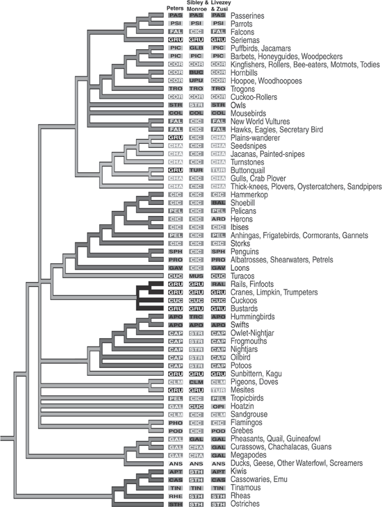
FIGURE 7.10 Results of a cladistic analysis of birds by Shannon Hackett and her colleagues, compared with the results of three earlier studies, from “A Phylogenomic Study of Birds Reveals Their Evolutionary History” (2008). (Reproduced with permission of the American Association for the Advancement of Science)
Two examples show how the ideas of phylogeny changed between the earlier studies of Sibley and colleagues (Sibley, Ahlquist, and Monroe 1988; Sibley and Monroe 1990) and those of Hackett and co-workers (2008) almost twenty years later. Ciconiiforms represent the first example, shown under Sibley and Monroe (1990) as a frequently repeated white CIC. Traditionally, this group included storks, herons, egrets, spoonbills, and ibises—generally large-billed, long-legged, larger wading birds. But to these, Sibley and his colleagues added a number of other groups, which because of their scattered positions on Hackett and her colleagues’ phylogeny obviously could not be monophyletic. One of the more curious ciconiiform cases that received some press attention involves New World vultures, traditionally placed with Old World vultures, hawks, and eagles, but instead Sibley and his colleagues found them to be in their greatly expanded ciconiiform order. As can be seen in figure 7.10, Hackett and her colleagues returned them to a position as being the nearest relatives to the hawks, eagles, and Old World vultures.
The second example involves the globally distributed flightless ratites—ostriches in Africa, kiwis in New Zealand, cassowaries and emus in Australia, and rheas in South America. Their monophyly has been questioned at times, but Sibley and his colleagues found them to be monophyletic with their nearest relatives, the flighted tinamous of South America. This would suggest that flightlessness originated once, and then ratites, both extant and extinct, distributed themselves around the southern continents as the southern supercontinent Gondwana broke apart. The findings of Hackett and her colleagues strongly questioned this result and in the process provided a case in which tree building showed not only how species are related but also some important evolutionary steps that occurred because of their new analysis. As seen in the base of their phylogeny, the flighted tinamous share a more recent ancestry with the common ancestor of New Zealand kiwis and Australian cassowaries and emus (see figure 7.10). They do not indicate whether they think their phylogeny argues that the ability for flight reemerged in tinamous or was lost three times, once each in the ostriches, rheas, and combined Australian–New Zealand clade. In another paper with eighteen authors (Harshman et al. 2008), most of whom also contributed to Hackett and colleagues (2008), the conclusions present a more emphatic result, as indicated by the title, “Phylogenomic Evidence for Multiple Losses of Flight in Ratite Birds,” with a major conclusion that “the most plausible hypothesis requires at least three losses of flight and explains the many morphological and behavioral similarities among ratites by parallel or convergent evolution” (13462) One can imagine that this did not make morphologists and behaviorists happy. This is but one example showing the importance of tree building in assessing evolutionary processes and not just patterns, especially following on earlier important, cladistically based biogeographers such as Brundin (1965, 1966).
The issues surrounding phylogenetic trees of birds pertain not only to who is related to whom, but to the times when various groups of birds originated. This brings us back to the arguments about the reliability and universality of the molecular clock, which, as discussed, appeared in a paper by Zuckerkandl and Pauling (1965b). Whereas arguments for the universality of rates of change of the molecular clock waned after 1965, arguments for some sort of so-called relaxed molecular clock became stronger, to the point that a clear disconnect arose between molecularly and anatomically based phylogenetic analyses and the resulting trees. Over time, more and more of a consensus arose between anatomy and molecules regarding the nature of bird relationships, but when the splitting of lineages occurred remains at an impasse, with most anatomically based phylogenies claiming that most orders of modern birds arose after the extinction of nonavian dinosaurs at the end of the Cretaceous period, some 66 mya. For example, Alan Feduccia (1995, 1996) argued that Neornithes, or modern birds, did not originate and radiate until after the Cretaceous–Paleogene (K–Pg) boundary. In what must be one of the more imaginative phylogenetic diagrams (figure 7.11A), Feduccia shows not only the origin and radiation of Neornithes after the K–Pg boundary but also a very substantial radiation and extinction of Enantiornithes (Archibald 2011). These are a curious lot; in fact, the name means “opposite birds.” Although enantiornithines certainly appear to have been ecologically diverse in the Late Mesozoic, there are only thirty named species, and to my knowledge there is only one named species from the latest Cretaceous, although two other unnamed forms occur (Longrich, Tokaryk, and Field 2011). This is a far cry from the radiation in Feduccia’s phylogenetic diagram that makes them a close second to neornithines, which are known from more than nine thousand species. Based on molecular and paleontological analysis, Alan Cooper and David Penny (1997) argued quite the opposite of Feduccia—not only that modern birds originated well before the K–Pg boundary (indicated by ~65 Ma on figure 7.11B), but that twenty-two lineages of modern birds crossed this boundary. The numbers given on this downward-opening phylogeny show various levels of confidence known as bootstrap values along each branch, where 100 is best. As these two phylogenies show, the issue of the timing of the origin of modern birds remains contentious. More recent studies (for example, Longrich, Tokaryk, and Field 2011) accept that fossils do indicate that neornithines existed in the Late Cretaceous, but the claim for a Late Cretaceous radiation of these modern birds as seen in Cooper and Penny cannot be supported by the fossil record (see figure 7.11B).
The issue of when modern mammals arose represents an even greater schism between paleontological and anatomical data, on one hand, and molecular data, on the other. The single greatest reason for this disagreement is that unlike more fragile birds, for which the fossil record remains relatively sparse and hence less defensible as a source of data, mammals left a far more extensive fossil record because of their more durable bones and teeth. By the mid-nineteenth century, scholars identified tiny fossil jaws and teeth from the Mesozoic era that today we would agree represent mammals. Sorting out how these might be related to modern mammals remained more questionable. By the time of Charles Darwin in the latter half of the nineteenth century, as in the two mammalian phylogenies in his letter to Charles Lyell in 1860, the concept of marsupial and placental mammals began to emerge, although Darwin could not decide whether marsupials and placentals shared a nonmarsupial/nonplacental common ancestor (see figure 4.12) or whether primitive marsupials were the ancestors of both marsupials and placentals (see figure 4.13). In his phylogeny, Ernst Haeckel (1866) seemed more certain of ancestry, showing marsupials (his Didelphia) as ancestors of modern marsupials as well as modern placentals (his Monodelphia), which arose somewhere in the Triassic period, if not before (see figure 5.4). Others speculated as well on the origin of modern mammalian groups; for example, Vladimir Kovalevskii’s (1876) phylogeny of hooved mammals shows a hypothetical Urungulata from the Late Cretaceous, which we now know existed as Protungulatum (see figure 5.2C) (Archibald et al. 2011). By the mid-twentieth century, there seemed little doubt that marsupials and placentals possessed long, separate evolutionary histories. If we consider only placentals, their phylogeny began to take on a particular shape based largely on the fossil record of the time that enabled the modern groups of placentals to be traced back to only the beginning of the Cenozoic era, now dated at about 66 mya, although a few ancestral lineages trickled backward into the Cretaceous—an explosive radiation based on the fossil record. This iconography occurs in trees by Alfred Romer from 1933 (see figure 6.7B) and 1971 (see figure 6.7C) that characterized the basic ideas of the time: that much of the radiation of modern placental mammals occurred after the extinction of the dinosaurs, although more ancient eutherian ancestors or cousins of the modern placentals had been recognized in the fossil record of both the United States and Mongolia by the early twentieth century. The knowledge of such Cretaceous eutherians expanded rapidly in the last third of the twentieth century.
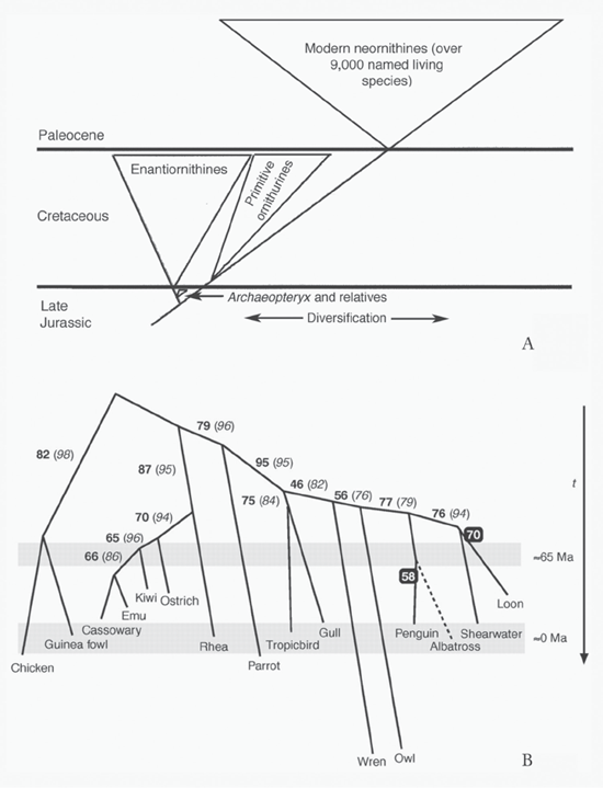
FIGURE 7.11 (A) Phylogeny, redrawn after one in Alan Feduccia’s “Explosive Evolution in Tertiary Birds and Mammals” (1995) and The Origin and Evolution of Birds (1996), arguing that Neornithes did not originate and radiate until after the K–Pg boundary, and for a very substantial radiation and extinction of Enantiornithes, from J. David Archibald’s Extinction and Radiation (2011); (B) Alan Cooper and David Penny’s downward-opening phylogeny, arguing for many lineages of birds arising before the end of the Mesozoic, from “Mass Survival of Birds Across the Cretaceous–Tertiary Boundary” (1997). ([A] reproduced with permission of Johns Hopkins University Press; [B] reproduced with permission of the American Association for the Advancement of Science)
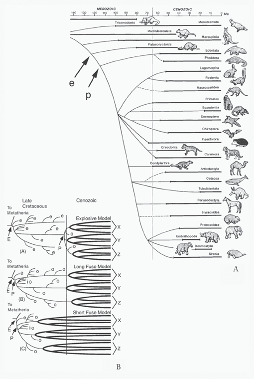
The advent of more sophisticated molecular techniques discussed earlier began rapidly to change the phylogenetic terrain. The vertebrate paleomammalogist Michael Novacek (1992) presented what at that time constituted the current state of affairs for eutherian and placental evolution in an aptly titled paper, “Mammalian Phylogeny: Shaking the Tree.” In his phylogeny, he shows modern orders of placentals, with the exception of the problematic Insectivora, going back to only the beginning of the Cenozoic (figure 7.12A, heavy lines), much as Romer (1933, 1971) presents, but with quite a new wrinkle. Using lighter solid lines, Novacek traces various lineages backward into the Cretaceous, joining to form various super- or interordinal groupings, but, as he fully acknowledges, the actual dates of these splitting events could be inferred only from the relationships of the clades and their known ages. Nevertheless, his educated guess placed the earliest of the placental splits at about 115 mya (indicated by arrow and p) and pushed back the origin of eutherians a few more million years to slightly over 120 mya (indicated by arrow and e). The abstract for the article clearly conveys the intended message and the then state of phylogenetic affairs: “Recent palaeontological discoveries and the correspondence between molecular and morphological results provide fresh insight on the deep structure of mammalian phylogeny. This new wave of research, however, has yet to resolve some important issues” (121). As Novacek relates in the article and shows on his phylogeny, as of 1992 various molecularly and morphologically based studies converged on the following ideas:
1. New World edentates (armadillos, sloths, anteaters) perhaps represent the earliest branching clade among placentals.
2. The basic relationships of the artiodactyls (cows, deer, sheep, pigs, camels) can be ascertained.
3. Artiodactyls and cetaceans cluster together separate of several other placental orders.
FIGURE 7.12 (A) Michael Novacek’s phylogeny showing eutherians (e [added]) and placentals (p [added]), in which modern orders of placentals go back to only the beginning of the Cenozoic (heavy lines), while some lineages date to the Cretaceous (light lines), joining to form various super- or interordinal groupings, from “Mammalian Phylogeny” (1992); (B) J. David Archibald and Douglas Deutschman’s names for three patterns of eutherian and placental evolution that had been recognized (E = origin of Eutheria; P = origin of Placentalia; e = eutherian but not placental lineage; o = extant placental order; io = interordinal placental groups), from “Quantitative Analysis of the Timing of Origin of Extant Placental Orders” (2001). ([A] reproduced with permission of the Nature Publishing Group; [B] reproduced with permission of Springer)
A clearer understanding of how the various modern orders of placental mammals related one to another and an idea of when these splittings might have occurred awaited newer molecular sequencing techniques. Already, however, the sort of trees that Romer showed, on one hand, and Novacek represented, on the other, portrayed two views of the timing of placental origination and diversification. In 2001, Douglas Deutschman and I named these two different views the Explosive and the Long Fuse models. The Explosive model, as in Romer’s trees, shows that placental mammals originated very close to either side of the K–Pg boundary (P in figure 7.12B), with modern orders appearing very soon after (o in figure 7.12B). Contrast this with the Long Fuse model, as in Novacek’s tree, which shows that placental mammals originated quite far back in the Late Cretaceous (P in figure 7.12B), but as in the Explosive model, modern orders appear near the K–Pg boundary (o in figure 7.12B).
A series of papers in the early twenty-first century offered new and sometimes startling phylogenetic results. William Murphy and colleagues (2001) used molecular data to argue that modern orders of placental mammals fall into four larger, superordinal groupings. Three of these groupings offered no great surprises, as they accorded in general with paleontological data (figure 7.13A), but the fourth, Afrotheria, was a surprise. It united typically African mammals, from aardvarks to elephants to golden moles, into one group. The analysis and phylogeny show this radiation of largely African mammals (see figure 7.13B), which had not been predicted on paleontological and morphological data, although sirenians, elephants, and hyraxes previously clustered with such data. Further, in the biogeographic tradition of Haeckel in the nineteenth century and Brundin in the twentieth, Murphy and his colleagues overlaid this superordinal phylogeny onto what was understood of the breaking apart of the southern supercontinent Gondwana to suggest how the phylogeny came to be (see figure 7.13C). They argued that placentals arose and began to divide into four superorders between 108 and 101 mya, in keeping with the splitting of Africa and South America between 120 and 100 mya. Certainly, then, their phylogenetic analysis argued for at least the Long Fuse model, according to which the placentals originated and began to diversify at least into superordinal groups in the Late Cretaceous (see figure 7.12A), but when modern orders of placentals arose remained an open question.
An article by Olaf Bininda-Emonds and colleagues (2007) used molecular data to present a supertree, meaning that it was constructed by clustering a series of smaller trees using various data sets. According to these authors, “The supertree contains 4,510 of the 4,554 extant species recorded…making it 99.0% complete at the species level” (507). They argued that not only did placentals and other modern mammals originate and split into superorders in the Late Cretaceous, but modern orders of mammals also appeared in the Late Cretaceous, well before the extinction of the dinosaurs some 66 mya. The authors not only dated the origination and earliest diversification of mammalian orders to some 93 mya, but also argued that mass extinction at the end of the Cretaceous did not have a major, direct effect on the diversification of modern mammals. This follows the pattern of the Short Fuse model of the origination and early diversification of all modern mammals within the Late Cretaceous (see figure 7.12B). The spiraling rather than tree-like phylogeny used by Bininda-Emonds and his colleagues, while not new or even a rare method for representation, certainly was chosen in part because of the need to show a considerable number of species (figure 7.14). The dashed circular line on the phylogeny marks the K–Pg boundary at about 66 mya. This means that not just the ancient ancestors of some families of living mammals but actual members of these families lived with dinosaurs—rats, mice, and beavers cavorted at their feet while camels shared their fields, and varieties of bats flew above them—a scenario that many biologists reject.
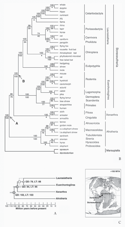
FIGURE 7.13 Using molecular data, William Murphy and his colleagues found (A) four major superordinal clades of (B) living placental mammals, which they argued (C) show a split following patterns of the breakup of Gondwana, from “Resolution of the Early Placental Mammal Radiation Using Bayesian Phylogenetics” (2001). (Reproduced with permission of the American Association for the Advancement of Science)
FIGURE 7.14 Spiraling phylogeny, based on molecular data, by Olaf Bininda-Emonds and his colleagues, arguing that not only did modern mammals originate and divide into superorders in the Late Cretaceous, but modern orders of mammals also appeared in the Late Cretaceous, well before the extinction of the dinosaurs (dashed circle), from “The Delayed Rise of Present-Day Mammals” (2007). (Reproduced with permission of the Nature Publishing Group)
The pendulum swung fully with a paper by Maureen O’Leary and colleagues (2013a). The authors combined morphological, or what they termed phenomic, characters in obvious apposition to genomic characters, along with molecular data. While the results shown in their phylogenetic tree did differ in some ways from those in earlier studies, the biggest furor resulted from marked differences in the timing of these evolutionary events (figure 7.15). Whereas Murphy and colleagues (2001) had placed at least the origin of placental superorders at about 100 mya and Bininda-Emonds and co-workers (2007) had further argued that modern orders of mammals appeared by 93 mya, O’Leary and her colleagues not only dated the origin of modern placental orders to after the K–Pg boundary, at some 66 mya, but also argued that placental mammals did not even appear until then. Thus, according to them, placentals arose some 36 million years later than Bininda-Emonds and his colleagues determined, not an insignificant interval, given that all researchers would agree that the remaining time span for placentals on Earth is some 66 million years in duration. In the O’Leary scenario, unlike that of Bininda-Emonds, the end of the Cretaceous had a profound effect on mammalian evolution, and contrary to that of Murphy, the breaking apart of Gondwana was not a factor in early placental diversification.
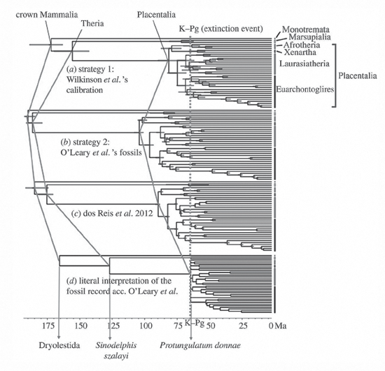
Any differences in their phylogenetic results and trees pale in comparison with the profoundly contrasting views of the timing of these events. For these varying interpretations, this difference of some 36 million years is far from insignificant, and much of it derives from divergent views about the importance of assuming or not assuming some sort of molecular clock (O’Leary et al. 2013b; Springer et al. 2013) as well as the way fossils can be used to calibrate age estimates for the various lineages. Mario dos Reis, Philip C. J. Donoghue, and Ziheng Yang (2014) presented a series of four trees showing identical evolutionary relationships among but greatly different timings for the origin of modern placental mammals (figure 7.16), echoing the older origination espoused by Bininda-Emonds and colleagues (2007) versus the more recent origination argued by O’Leary and co-workers (2013a). In figure 7.16, note the position of the line labeled “Placentalia,” which varies from almost 100 mya to about 65 mya in the placement of the time of origin for this group. Regardless of whose interpretation of the timing of the origination of modern placental mammals is correct, we see an important use of phylogenetic trees (or cladograms) to present differing ideas about origination times. This recalls Haeckel’s (1866) use of trees to offer various hypotheses about the origin of life (see figure 5.3). Once again, we see trees showing something beyond evolutionary relationships.
These ongoing disputes about the timing of major evolutionary events occur for all major groups, not just for the study of mammalian evolution and diversification. These considerable differences in opinion concerning the timing of events using various phylogenetic analyses, whether they deal with the origin of multicellular life or the origin and diversification of modern birds and mammals, will assuredly continue. Notwithstanding, the question of timing is not the only issue dogging tree building; the more profound question arises as to whether a tree is even a reasonable visual metaphor for the history of life.

FIGURE 7.15 Phylogenetic tree by Maureen O’Leary and her colleagues, based on combined phenomic and genomic characters, differs in some ways from earlier diagrams, primarily in the placement of the origin of placentals, including all extant orders, after the K–Pg boundary some 66 million years ago, from “The Placental Mammal Ancestor and the Post–K-Pg Radiation of Placentals” (2013). (Reproduced with permission of the American Association for the Advancement of Science)
FIGURE 7.16 Four phylogenetic trees by Mario dos Reis, Philip C. J. Donoghue, and Ziheng Yang, showing the same evolutionary relationships among but very different times for the origin of Placentalia, ranging from almost 100 million years ago to about 65 million years ago, from “Neither Phylogenomic nor Palaeontological Data Support a Palaeogene Origin of Placental Mammals,” Biology Letters 10 (2014):fig. 1. (Reproduced with permission of the Royal Society)
The Molecular Tree Becomes Tangled
The advent of molecular systematics showed that at least for simpler organisms, such as bacteria, the tree became a tangled, thorny bramble menacing results everywhere: “It is interesting to contemplate a tangled bank, clothed with many plants of many kinds” (Darwin 1859:489). When Darwin penned these words in the final sentence of On the Origin of Species, he was reflecting on complex interaction of species in ecological relationships that produced evolutionary change over millions of generations. He could not have realized just how tangled the evolutionary history of many species could be, enough in fact for some biologists to cast serious doubt on the tree metaphor for the history of life. Darwin certainly knew of and wrote about at least one form of evolutionary entanglement, hybridization, including a complete chapter about it in On the Origin of Species. Nonetheless, he did not fully know the importance of hybridization among complex organisms, particularly in the speciation process of angiosperms, or flowering plants. Darwin expressed great consternation concerning the evolutionary history of angiosperms, which he termed an “abominable mystery.” He struggled with the idea that the origin and diversification of flowering plants might be both sudden and rapid, quite against his view that evolution was slow and stately—natura non facit saltum (nature does not make a leap) (Friedman 2009).
Darwin would be thrilled and possibly even not surprised to learn that perhaps all angiosperms experienced some form of hybridization during their evolutionary history, and angiosperms may number as many as 400,000 species (Soltis and Soltis 2009). Figure 7.17A shows a simple example of how hybridization may be represented in a tree, somewhat resembling how a pedigree of an offspring from two parents might look (Linder and Rieseberg 2004). In this case, however, species X and Y hybridize to produce species B, with the parent species continuing as species A and C. But what, then, would the more complicated tree of life look like with rampant crossing, such as between angiosperm species? Two studies of the numerous examples show what such trees look like. The annual sunflower Helianthus appears in such a tree (see figure 7.17B), using combined molecular data from both the chloroplast and the nucleus (Gross and Rieseberg 2005). Two species, H. petiolaris and H. annuus, repeatedly show crosses in various environments, resulting in hybrids that fare better than either parent in such environments. The numbers above the horizontal lines show the number of mutations leading to each clade, and the numbers below indicate a measure of confidence in that particular clade, in this case using a technique known as bootstrapping, in which 100 is the maximum value. Once one knows what is being shown, the hybridization events in this tree become quite clear. The second, even more complex example involves the small annual plant Clarkia, named for the explorer William Clark of Lewis and Clark fame and found mostly in the western United States (Futuyma 1986). Figure 7.17C shows the intricate phylogeny and hybridization within this genus. For the parent species, the numbers refer to the number of chromosomes in the gametes, which are not always the same in both parent species, in turn giving rise to the number of chromosomes in the descendant hybrid (for example, C. mildrediae-7 and C. virgata-5 yielded C. rhomboidea-12). Interestingly, the sort of analysis shown in this phylogeny allows a prediction of what the gamete chromosomal number would be for unknown ancestors, indicated by numbers unaccompanied by names. Although seemingly a tangled network, this powerful phylogenetic hypothesis uses a tree to argue in which direction and by which means (hybridization in this case) evolution has traversed.
Because the very basis of inheritance was unknown to Darwin and most others in the nineteenth century, they could not have conceived how important other methods of genetic transfer were between organisms of the same and different species. And anyway, how would one show this on the traditional metaphorical tree of life? Although various processes had been known for some time, dubbed “reticulate evolution” for obvious reasons, the issue came to a head in 1999 when the biochemist W. Ford Doolittle (b. 1942) published two of what he termed “crude sketches[s].” Crude they were, but powerful as well in their simple message—much reticulate evolution occurred in the history of life, especially the early part, in the form of horizontal or lateral gene transfer. This greatly complicates our attempts to reconstruct the history of life on Earth. If not a tree, what metaphor should be used?

FIGURE 7.17 (A) C. Randal Linder and Loren Rieseberg’s simple example of how hybridization may be represented in a tree, from “Reconstructing Patterns of Reticulate Evolution in Plants” (2004); (B) Brianna Gross and Rieseberg’s phylogenetic analysis of the annual sunflower Helianthus, using combined molecular data from both the chloroplast and the nucleus, showing repeated hybridization from H. petiolaris and H. annuus, from “The Ecological Genetics of Homoploid Hybrid Speciation” (2005); (C) Douglas Futuyma’s more complex example, showing the intricate phylogeny and hybridization within the genus Clarkia, from Evolutionary Biology (1986). ([A] reproduced with permission of the Botanical Society of America; [B] reproduced with permission of the Journal of Heredity and L. Rieseberg; [C] reproduced with permission of Sinauer)
Doolittle’s (1999) first sketch represented what at the time was “commonly taken as a representation of organismal phylogeny and the basis for a natural classification” (2125). At the top of this sketch, we see the three so-called domains to which all but viruses were believed to belong (figure 7.18A). In the diagram, Bacteria encompass what we traditionally consider bacteria to be, such as Escherichia coli, commonly called E. coli, which strikes fear into the hearts, or guts, of many people, even though many strains are harmless or even beneficial. In this classification, Bacteria also include a great variety of other prokaryotic microorganisms, such as blue-green algae, all of which lack a nucleus (Gk. karyon) or other cellular organelles, such as mitochondria. Archaea, once thought to be a form of bacteria and far less known to most people, are also prokaryotic microorganisms, many of which live in extreme conditions—the original thrill seekers. The third domain, Eukarya or Eukaryota, whose cells possess a nucleus and cellular organelles, includes animals, plants, and fungi, as shown in Doolittle’s sketch. Note, however, that two branches of Bacteria trace to Eukarya. Doolittle did not intend to indicate, as a nineteenth-century biologist such as Haeckel might have meant, that these lineages had separately evolved into eukaryotes but something more radical, first considered at the beginning of the twentieth century but not validated until the 1960s. In 1967, the biologist Lynn Margolis (1938–2011) provided microbiological evidence that early in evolutionary history, eukaryotic cells had incorporated various bacteria into themselves—mitochondria in animals and plants, and chloroplasts in plants—which became known as the widely accepted endosymbiotic theory (Sagan 1967). Thus by at least the mid-twentieth century, there was some inkling that the tree as a metaphor for the history of life existed on borrowed time, at least for part of evolutionary history.
It was Doolittle’s second “crude sketch” that brought to the fore just how complicated the history of life on planet Earth really is (see figure 7.18B). Granted, much of this entanglement may have begun early in the history of life, but “early” in the frame of Earth’s history represents perhaps 4 billion years, or only three-quarters of the time that life has existed on this planet, compared with the possibly 1 billion years that eukaryotes have been around. Instead of just two arrows heading from bacteria to eukaryotes, the tree now resembles nothing less than a tangled mess of interdomain relationships. It became clear that during the history of life, the basal members of these domains began to sort themselves out but along the way also cross-shared considerable chunks of their genomic and cellular machinery. The entanglement of early life means that the interrelationships of the three domains, and whether the contents of each domain are correctly assigned, remain an unsolved puzzle.

FIGURE 7.18 W. Ford Doolittle’s sketches represented (A) what was considered the common view of organismal phylogeny, compared with (B) what was being revealed about horizontal gene transfer between many simpler species, from “Phylogenetic Classification and Universal Tree” (1999); (C) Carl Woese and George Fox’s three domains, before the name change from Archaebacteria to Archaea, from Woese, “Bacterial Evolution” (1987); (D) the navigational tree-like figure from the Tree of Life (ToL) Web Project. ([A] and [B] reproduced with permission of the American Association for the Advancement of Science; [C] reproduced with permission of Microbiology and Molecular Biology Reviews; [D] reproduced with the permission of Nick Kurzenko)
The three domains were not even recognized until 1977, when Carl Woese (1928–2012) and his colleague George E. Fox (b. 1945) distinguished a new group based on 16S ribosomal RNA (the molecular scaffold in Archaea and Bacteria used for synthesizing proteins), which they first called Archaebacteria but later changed to simply Archaea to make it clear that this new domain was not a form of bacteria. Woese (1987) presented the major groups as an unrooted network in a review paper in which Archaea was still referred to as Archaebacteria (see figure 7.18C), rather than a tangled tree as in Doolittle’s (1999) figure (see figure 7.18B). Even the rooting of the tree cannot be done with any certainty because an outside nonliving comparison is needed—a rock, for instance. Aristotle (1991, 2007) and Charles Bonnet (1745) had it more right than wrong in placing inanimate material at the base of all life or, more correctly, as the sister group to life.
The most current treatments of how the relationships of life on Earth should be represented grapple with such questions as rooting the tree of life and the complexities of tree reconstructions caused by horizontal gene transfer. A special issue of the journal Biology & Philosophy titled “The Tree of Life” examined “scientific, historical and philosophical aspects of debates about the Tree of Life, with the aim of turning these criticisms towards a reconstruction of prokaryote phylogeny and even some aspects of the standard evolutionary understanding of eukaryotes” (O’Malley, Martin, and Dupré 2010:441). Although the contributors varied considerably in their views about the metaphorical relevance of a tree of life image, the journal certainly placed the issues front and center.
In the rapidly changing world of the Internet, a number of sites examine the tree of life, with the Tree of Life (ToL) Web Project (Maddison and Schulz 2007; Maddison, Schulz, and Maddison 2007), an unarguably major one. Its home page is graced by a visually poetic image, which the authors emphasize is a greatly simplified illustration that serves a navigational purpose (the tree is a table of contents of sorts) (see figure 7.18D). The authors stress that the earliest history of life is obscure in the diagram because evidence indicates that rather than a single primordial cell, the first organisms possessed loosely constructed cellular organization and frequently exchanged genetic material; perhaps the origin of life cannot be seen as monophyletic or polyphyletic but as a prebiotic amalgam exchanging information. Even later, after the establishment of distinct genetic lineages, these exchanges of genetic material continued, which the diagram indicates by lines connecting distant branches of the tree. Whereas horizontal gene transfer clearly helped define Eubacteria and Archaea, its significance for eukaryotic evolution becomes less clear with the exception of eukaryotes’ acquisition of organelles such as mitochondria and chloroplasts by the engulfment (endosymbiosis) of bacteria. As shown in figure 7.18D, the relative magnitudes of various clades distort an accurate representation of diversification; if not, arthropods (notably insects) would greatly dominate the figure. Based on recent estimates of the true diversity of bacteria, protists, fungi, and nematodes, the remainder of the tree would be filled by branches for these groups; vertebrates and plants would be barely visible to the naked eye. Once again, the importance of humans is placed in its correct perspective.
Coming Full Circle
Near the end of the twentieth century, with a combination of new and faster methods to extract and sequence molecular data combined with ever accelerating computer power, the phylogenetic trees began to take on a life of their own—no longer simply bifurcating diagrams. Additionally, with the simple yet profound realization that relative splitting on a tree, and not nearness of groups or how high or low on a tree they rest, determines evolutionary relationship, a new freedom in how to express trees arose. I use the word “tree” broadly because many of the new diagrams are anything but trees in a traditional sense. As seen, they vary from trees to circles to webs. All of them are the same in using relative splitting of groups or clades to show evolutionary relationships, but some use anatomy, others use molecular data, and others use both. In this way, these figures are the same. In part, some of the new shapes arose out of necessity to conserve space yet present as much information as possible.
The traditional tree form, even if festooned with fossil species, presents a basic triangular shape that wastes space on the page, but less so with a circle or, more accurately, a spire on which the relationships spiral inwardly to the origin with the various taxa arrayed around the circumference. A well-known version of this sort of figure appeared in Science (Pennisi 2003), by the molecular systematist David Hillis (b. 1958) and colleagues (figure 7.19A). This densely packed figure shows three thousand named species throughout all the kingdoms of extant life and is best viewed when scaled to a diameter of 5 feet (1.5 m). Hillis writes, “The number of species represented is approximately the square-root of the number of species thought to exist on Earth (i.e., three thousand out of an estimated nine million species), or about 0.18% of the 1.7 million species that have been formally described and named” (Hillis, Zwickl, and Gutell). Relative proportions of various groups skew toward eukaryotes, including us. Even then, it is humbling for Homo sapiens to be one infinitesimal smudge labeled “You are here.” It is reminiscent of the famous photograph taken from Voyager 1 near the edge of the solar system showing Earth as a small pinprick of light.
Although intriguing in their form, these circular representations of life’s diversity are not new. A favorite is the frontispiece of Heinrich Bronn’s (1850–1856) atlas for the third edition of his book Lethaea geognostica (see figure 7.19B). In the original edition, Bronn (1837–1838) used the more traditional paleontological chart showing older fossils at the bottom and younger ones near the top (see figure 3.13B), but in this over 150-year-old version he attempted, as do systematists of today, to save space by using a circular form, with the oldest ages of Earth near the center and life-forms radiating outward to the circumference. This is by no means a phylogeny but a circular paleontological range chart, but recall that in 1858 Bronn published only the second tree-like figure, clearly advocating evolutionary descent; Jean-Baptiste Lamarck’s (1809) version was the first. One can imagine that if Bronn had not died in 1862, we might have seen more evolutionarily based paleontological diagrams from him. Near the outer edge of the circle, Bronn indicates the number of extant species for that particular group, with a total of more than 173,000, a far cry from the millions of species we now believe to exist, but nevertheless impressive. Of course, unlike the diagram of Hillis and his colleagues (see figure 7.19A), humans (Menschen) rest at the top of Bronn’s circle, crowned by a crucifix and overseen by the eye of God. No matter how one chooses to portray our position in nature, we are part of it. Our interpretations of this position, at times messy and sometimes downright nasty, help us divine who we think we are and where we believe we belong within the scheme of things. It is an ongoing process.
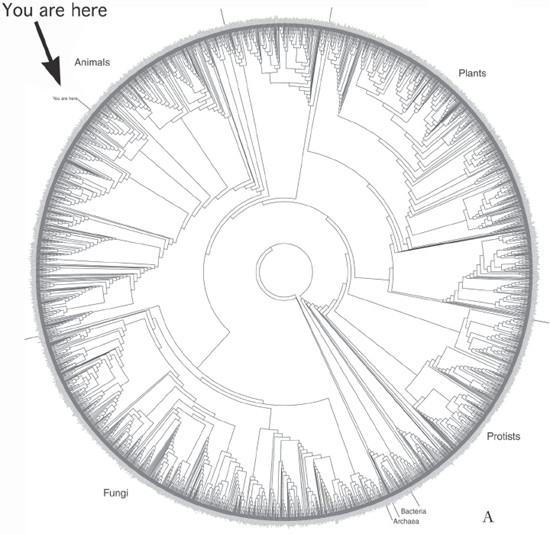

FIGURE 7.19 (A) Spiral phylogeny by David Hillis, Derrick Zwickl, and Robin Gutell, showing three thousand named species throughout all kingdoms of extant life; (B) frontispiece of Heinrich Bronn’s atlas for Lethaea geognostica (1850–1856), a circular paleontological range chart (not phylogeny) of life’s diversity. ([A] David Hillis, Derrick Zwickl, and Robin Gutell, University of Texas, are thanked for allowing the use of the spiral phylogeny)