Pollsters have been seeking Americans’ opinions about their presidential choice for over two-thirds of a century. The practice has now intensified to the point where hardly a day passes during an election year without encountering results of new presidential polls, often from multiple organizations. In these so-called trial-heat polls, citizens typically are asked how they would vote “if the election were held today,” with some differences in question wording, although in some early polls respondents were asked who they “would like to see win.”
The first scientific polls to ask presidential preferences were conducted in 1936; their architects were the now-famous trio of Crossley, Roper, and Gallup.1 By 1944, Gallup was conducting trial-heat polls on a regular basis. In that election year alone, Gallup asked twenty-eight different national samples of voting-age adults about their preference for the major-party presidential candidates—Franklin D. Roosevelt and Thomas E. Dewey. Since then, Gallup has conducted polls on a monthly or more frequent basis in every presidential election year.
By 1980, each of the leading broadcast networks (ABC, NBC, and CBS) were conducting surveys. Some newspaper organizations were too. The number grew through the 1980s. Independent organizations joined the ranks, and the proliferation of cable news networks added still more. In 1992, no less than 22 organizations conducted at least one poll. In 2000, more than 36 different organizations did. Over 19 fielded at least five polls. Five conducted tracking polls during the last month of the campaign, putting them in the field every day. The PollingReport.com website showed results from some 524 national polls of presidential election preferences during the 2000 election year. By 2008 there were more than 800 national polls.
Improved polling technology—especially the switch to telephone—accounts for much of the growth in presidential polling. Until well into the 1980s, most polls were conducted in person, as interviewers met with respondents in their homes. Given the logistics of interviewing a representative national sample in person, in-home polls typically were conducted over many days, over a window as wide as two weeks. By the mid-1970s, some pollsters were turning to telephone interviewing, which allowed quicker results at much less cost. By the mid-1990s, the transition to telephone was almost complete. One result is the greater density of polling we see today. During recent presidential election years, hardly a day passes without new presidential polls, often from multiple organizations.
The twenty-first century has seen still further technological innovations that have allowed quicker and cheaper polling. We refer to the rise of Internet polls—in which respondents are recruited for web-based interviews—and interactive voice response (IVR) polls—in which people are interviewed over the telephone but by recorded voices rather than live interviewers. For this book, we ignore polls conducted with the use of these new technologies.2 The reason is not that they are certifiably wrong or inferior to live-interviewer polls, because that is not the case. Internet and IVR polls sometimes give results that differ from those of live-interviewer polls, however. When comparing polls historically, we conclude that it is safer to only include the live-interviewer polls from recent presidential races. The density of polling using this approach in recent elections is more than sufficient for our analysis.
Concern about comparability across time also compels a further restriction of our analysis. We start our analysis in 1952 and ignore earlier presidential polls from 1936 to 1948. Before 1952, pollsters often employed the flawed “quota-sampling” method, which allowed interviewers the freedom of whom to interview as long as they were within designated demographic quotas. It was the bias from quota sampling that misled some pollsters to predict Dewey would defeat Truman in 1948. Since 1952, the samples for national presidential polls have been drawn using some variant of random assignment, typically “multistage random samples.”3 The theory of random assignment is that it allows every voter (or citizen) an equal chance of inclusion in the survey.
To summarize, our focus is on polls conducted by survey organizations using live interviewers and beginning with the 1952 presidential election, when quota sampling had been displaced by variants of random sampling.
Employing a cutoff of 300 days before the election, roughly the beginning of the election year, we consider all live-interviewer polls involving the eventual major-party candidates. Using these criteria, we have located what we believe to be all of the available national polls of the presidential vote division that included the actual Democratic and Republican nominees for the fifteen elections between 1952 and 2008. In analyzing these polls, we ignore differences in question wording. Lau (1994) shows that variation in question wording has little bearing on trial-heat results.4 Until 1992, the data are mostly from the vast Roper Center’s iPOLL database, the standard archive for such data. We also supplemented using the Gallup Report, the now-defunct Public Opinion, and the more recently defunct magazine Public Perspective. In 1996, the data were drawn primarily from the also defunct PoliticsNow website, supplemented by data from the Public Perspective and the iPOLL database (see Erikson and Wlezien 1999). Beginning with the 2000 election, the data are from PollingReport.com and the iPOLL database. The amassing of data is only the first step. Decisions are required regarding how the data set is put together. We identify three concerns and our solutions.
First, although our interest is in the support for the two major-party candidates, we have to deal with surveys that include minor-party candidates among their choices. When a survey organization asks its trial-heat question two ways—with and without minor-party candidates on their ballots—we use the results without the minor-party candidates. Where the organization only offers respondents a choice among three or more candidates, we include the poll but only count the major-party choices.
Second, in recent years—especially since 1992—survey organizations report multiple results for the same polling dates, reflecting different sampling universes. For example, early in the election year, Gallup may report results for samples of adults on the one hand and registered voters on the other. Later in the election year, they may report results for samples of registered and “likely” voters, where the later focuses only on those considered likely to vote.5 Clearly we don’t want to count the same data twice, so we use only the data for the universe that seemingly best approximates the actual voting electorate. Where a survey house reports poll results for both an adult sample and a registered voter sample, we use data from the latter. Where a survey house reports poll results for both registered voters and a sample of likely voters, we use data from the latter.6
Third, especially in recent years, survey organizations often report results for overlapping polling periods. This is understandable and is as we would expect where a survey house operates a tracking poll and reports three-day moving averages. Respondents interviewed today would be included in poll results reported tomorrow and the day after, and the day after that. Clearly, we do not want to count the same respondents on multiple days, and it is very easy to avoid. For the hypothetical survey house operating a tracking poll and reporting three-day moving averages, we only use poll results for every third day.
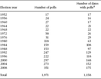
Applying these three basic rules has dramatic effects. Consider the 2000 election year. Recall from above that the PollingReport.com website contained results for some 524 national polls of the Bush-Gore (-Nader) division reported by different survey organizations. Eliminating results for multiple universes and the overlap in polling periods leaves only 295 separate national polls. For the period 1952–2008 we identify 1,971 different polls. The polls are not evenly distributed across elections and cluster in more recent years. Table 2.1 summarizes the data. Here we see that more than 90 percent of the polls were conducted in the eight elections since 1980. From 1980 through 2008, the number of polls averaged 225 per election. For the period before 1980, we have only 25 polls per election on average. Thus, the data offer much more frequent readings of electoral sentiment for the last six elections. Even in these recent years, the polls tend to cluster late in the electoral seasons, especially after Labor Day, when the general election campaign begins in earnest.
Most polls are conducted over multiple days. The median number of days in the field is 3 and the mean 3.75, though there is a lot of variance here—the standard deviation is 2.83 days. We “date” each poll by the middle day of the period the survey is in the field. If a poll is conducted during the three days between June 12 and June 14, we date the poll June 13. For surveys in the field with an even number of days, the fractional midpoint is rounded up to the following day.
For days when more than one poll result is recorded, we pool the respondents into one poll of polls. With the use of this method, the 1,971 polls allow readings (often multiple) for 1,158 separate days from 1952 to 2008 (see table 2.1). Since 1980, we have readings for 125 days per election on average, more than one-third of which is concentrated in the period after Labor Day. Indeed, we have a virtual day-to-day monitoring of preferences during the general election campaign for these years, especially for 1992–2008.
It is important to note that polls on successive days are not truly independent. Although they do not share respondents, they do share overlapping polling periods. That is, the polls on each particular day combine results of polls in the field on days before and after. Readings on neighboring days thus will capture a lot of the same things, by definition. This is of consequence for an analysis of dynamics, as we will see.
Table 2.1 Summary of presidential polls within 300 days of the election
a The variable indicates the number of days for which poll readings are available, based on an aggregation of polls by the mid-date of the reported polling period. Counts represent only live-interview polls involving the two major-party candidates.
Figure 2.1 and 2.2 present the daily poll-of-polls for the final 300 days of fifteen presidential campaigns. For the quick overview, figure 2.1 displays all the polls over fifteen years on the same page for ready comparison. Figure 2.2 displays the data in larger scale over several pages. In each instance, the graphs depict the Democratic share of the two-party vote intention, ignoring all other candidates (such as Nader in 2000), aggregated by the mid-date of the reported polling period. To be absolutely clear, the number on a particular day is the Democratic share of all respondents reporting a Democratic or Republican preference in polls centered on that day, that is, we do not simply average across polls.7 Where possible, respondents who were undecided but leaned toward one of the candidates were included in the tallies.
To enhance comparability across years, in figure 2.1 we subtract out the actual Democratic share of the two-party vote; thus, the numbers in the figure reflect the degree to which poll results differ from the final vote. A positive value indicates Democratic support that is above what we observe on Election Day, while a negative value reveals support that is below the Democratic candidate’s ultimate vote share. Ignoring the scattering of trial heats conducted in the year prior to the election, we concentrate solely on polls over the final 300 days of the campaign.
Figure 2.1. Trial-heat preferences for the final 300 days of the campaign, 1952–2008: A global view.
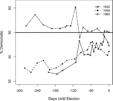
For the larger set of fifteen graphs in figure 2.2, the scaling is the percentage of Democratic rather than the deviation of the Democratic vote from the outcome. We group the fifteen elections into five graphs, with each showing the time series of the polls for three consecutive elections, starting with 1952, 1956, and 1960. The graphs show the final vote divisions as solid dots at 0 days before the election.
As can readily be seen from a perusal of figures 2.1 and 2.2, the daily poll-of-polls numbers exhibit considerably more within-year variance in some years than in others. Consider first some instances in which change was clearly evident. In 1992, the polls began somewhat favorable to President George H. W. Bush but then surged dramatically toward Democrat Bill Clinton after the Democratic National Convention, which was followed by tightening at the end of the race. The polls for 1980 show a similar degree of movement, with President Carter’s vote declining, then spiking upward, and fading at the end as he lost to Reagan. Interestingly, these were both elections in which the incumbent president sought and lost reelection. The other extreme is depicted by the polls of 1996 and 2004, when the incumbent presidents (Clinton and G. W. Bush) sought reelection and emerged victorious. In each instance, the polls were nearly constant, as shifts in voter sentiment were limited to a very narrow range. The 2000 G. W. Bush–Gore election and the 2008 McCain–Obama election are somewhere in between those two extremes. Real differences clearly exist across election years in terms of the volatility of voter preferences.
Figure 2.2A. Trial-heat preferences for final 300 days of the campaign, 1952–60. Observations represent daily polls of polls. The Election Day results are on the far right.
Figure 2.2B. Trial-heat preferences for final 300 days of the campaign, 1964–72. Observations represent daily polls of polls. The Election Day results are on the far right.
Figure 2.2C. Trial-heat preferences for final 300 days of the campaign, 1976–84. Observations represent daily polls of polls. The Election Day results are on the far right.
Figure 2.2D. Trial-heat preferences for final 300 days of the campaign, 1988–96. Observations represent daily polls of polls. The Election Day results are on the far right.
Figure 2.2E. Trial-heat preferences for final 300 days of the campaign, 2000–2008. Observations represent daily polls of polls. The Election Day results are on the far right.
Just as the within-year variances of the poll time series differ from election to election, the within-year variances of polls also differ from one time period to another over the campaign cycle. The time serial variance in the polls drops noticeably as the election cycle unfolds. This compression of variance is particularly pronounced after Labor Day, the unofficial beginning of the fall campaign. Figure 2.3 zooms in on this period and displays the daily poll-of-polls for the final 60 days of the campaign. (With the magnification, the range of the y-axis is now half of that shown in figs. 2.1 and 2.2.) On average, the variance of vote intentions as measured by polling in the fall is only about one-third of the variance for observations over the campaign’s previous 60 days. As we will see, much of the volatility of the polls is concentrated in the run-up to the fall campaign (including the period of the party conventions), not the fall campaign itself. We return to this point shortly.8
Figure 2.3. Trial-heat preferences for final 60 days of the campaign, 1952–2008.
In discussing trial-heat polls, we distinguish between the polls, which we observe directly from survey samples, and the underlying unobserved electoral preferences among the universe of potential voters. The observed divisions in trial-heat polls represent a combination of true preferences and survey error. By “true” preferences we mean the average response to the poll question among the universe of potential voters—the outcome of a hypothetical election conducted on that day. Of course our surveys do not perfectly reflect true preferences, because surveys are based on samples. Even if the electorate’s net true preferences remain unchanged over the course of a campaign, poll results will bounce around from day to day simply because of this survey error. This occurrence complicates any analysis using aggregate polling data.
There are different types of survey error; see Groves (1989) for a very thorough classification. The most basic and familiar of these is random sampling error, the variation in results that reflects the subset of people included in the sample. With the use of random sampling, the subset of people differs from sample to sample. The properties are well known, and we can provide reasonably accurate estimates of this error.
We cannot literally separate survey error from reported preferences. By applying long-established principles of statistics, however, we can estimate the proportion of the variance of the observed preferences that is due to true preferences and the remaining proportion that is due to survey error. If we assume random sampling (or its equivalent) by pollsters, the answer is easy to compute. We start with the observed variance in the polls. The observed variance can be daily variation in observed preferences over a specific time period, for example, over the final 30 days of the 2008 campaign. Or it could be yearly variation in the observed preferences over a specific cross-section, for example, preferences in the final week of each election. Statistically, the observed variance is the mean squared deviation of poll results from the observed mean. Then we estimate the error variance—the mean squared error per survey. The true variance is simply the subtraction of the error variance from the observed variance. The surplus (observed minus error) variance equals the true variance of presidential preferences, discounting for survey error.
But how do we estimate the sampling error? Assuming random sampling, for each daily poll-of-polls the estimated error variance is  , where p = the proportion voting for the Democratic candidate rather than the Republican. (Whether p designates the Democrat or Republican obviously does not matter.) Thus, when the size of the sample goes up, the estimated error variance goes down. When the race gets closer, the estimated error variance goes up. For instance, if the polls are 60–40 from a sample of 1,000 voters, we estimate error variance to be .6(1 − .6)/1,000, or .00024. If we use percents instead of proportions, the number would be 2.4 percent. If the result from a sample 1,000 is 50–50, we estimate error variance to be slightly larger, at .00025, or 2.5 in percentage terms. If the same result obtains from a sample of 2,000, we would estimate the error variance to be .000125, or 1.25 percentage points.
To illustrate, we focus only on polls conducted during the final 60 days of the campaign, or roughly from Labor Day to Election Day, when polling is most regular. For the value of p we take the observed Democratic proportion of major-party preferences in the poll. For N we take the number of respondents offering Democratic or Republican preferences. This gives us the estimated error variance for each daily poll-of-polls. The error variance for all polls-of-polls for the last 60 days in each election year is simply the average error variance. The total variance is observed from the variance of the poll results themselves. The estimated true variance is the arithmetic difference:
Estimated true variance = total variance − error variance.
The ratio of (estimated) true to total variance is the statistical reliability. The estimates for the final 60 days of fifteen campaigns are reported in table 2.2.
The table suggests that the true variance differs quite a lot across election years. Note first that in two election years—1960 and 1964—the observed variance is actually less than we would expect from random sampling and no true change. The 1960 contest was close throughout the last 60 days, perhaps never truly straying from the 50–50 margin ending in the outcome in which Kennedy defeated Nixon by a whisker. Quite plausibly, virtually all of the fluctuation in the 1960 horserace observed at the time was simply the result of sampling error. By similar reasoning, the 1964 horserace also was a virtually constant voter verdict—this time Johnson decisively defeating Goldwater. In these two contests, it is conceivable that few individuals changed their preferences during the fall campaign.
By our estimates, the largest true variance occurred in 1968, 1980, and 2000. In these elections, 75 percent or more of the observed variance was true variance. A true variance of 6.5 (2000) to 9.6 (1968) is indicative of a range of about 10 to 12 percentage points over the last 60 days of these campaigns. Clearly, the electorate’s aggregate vote intentions changed considerably during these presidential campaigns.
Table 2.2 Variance of daily trial-heat polls within 60 days of the election, 1952–2008

a For the calculations of means, the estimated true variance and reliability in 1960 and 1964 are considered to be 0.
It is tempting to speculate on different possible explanations for the variation from election year to election year in the actual volatility of the intended vote. One likely culprit is variation in voters’ prior knowledge about the candidates. Where there is an incumbent, things should be less volatile. Where the challenger is well known, the volatility should be lesser still. Thus, the thinking goes, we should expect little change in the polls during 1996 because Clinton and Dole were seemingly known quantities. Indeed the imputed true variance in 1996 was slight. In contrast, 1980 should be volatile because voters were trying to figure out Reagan. And this was one of the most volatile election campaigns. By our reasoning, it is easy to explain the volatility of 2000, when nonincumbent Gore faced the relative newcomer Bush. This reasoning fails in other instances, however. In 2004, for instance, polls were very stable even early in the election year as voters were asked to decide between a known, President G. W. Bush, and a newcomer to the national scene, Senator John Kerry. Earlier, polls moved around considerably in 1956, when Eisenhower and Stevenson were well known, but did not in 1960 and 1976, when the voters were learning about Kennedy and Carter, respectively. Thus, we conclude that the degree of volatility is not easily explainable, at least given the conventional wisdom.9
It should be sobering that, on average, the reliability of fall polls is a mere .45. This means that a bit less than half (45 percent) of the observed variance in the polls during the fall campaign is real, and a bit over half is sampling error. Even this estimate probably is generous regarding the accuracy of polls. By assuming simple random sampling, we ignore design and house effects. Design effects represent the consequences of departing in practice from simple random sampling, due to clustering, stratifying, weighting, and the like. House effects represent the consequences of different houses employing different methodologies and can reflect a variety of factors.10 Poll results vary from one day to the next in part because polls on different days are conducted by different houses (also see Wlezien and Erikson 2001). The point is that there is a lot more error in survey results than just sampling error.11
What is clear from our analysis is that the electorate’s aggregate preferences typically do not vary much over the fall campaign. We can put a number on the likely range in true preferences over the course of the fall campaign. Statistically, the range (from high to low) around the mean will be approximately plus or minus two standard deviations. From table 2.2 we see that the estimated mean true variance is 2.30 percentage points, so the corresponding standard deviation (the square root of the variance) is .52 points. This implies that for the average fall campaign, the maximum range of aggregate preference has been about 6 percentage points. As we discuss further in chapters 4 and 5, only a small percentage of the vote is at play during the autumn in a typical election year.
In assessing the variance of voter preferences, we are not limited to considering only the final 60 days of the campaign. In this section we examine the variance of the time series of voter preferences during earlier time segments of the campaign. Here we are interested in how the stability of preferences tends to vary with the point in the election cycle. Are preferences more changeable at some points than at others? Again, we adjust for sampling error. We subtract out variance owing to sampling error and assess the degree of (estimated) true variance in preferences in the different periods of each campaign. Then we “average” the variance by both period and election.
Table 2.3 summarizes this analysis, showing the median sampling-error adjusted within-election-year variance (across the fifteen elections) for a staggered series of 60-day time segments. The numbers in the table are what we find in a typical election year. Note the dramatic differences in the variances from one period to the next. The variance is lowest at 120 to 180 days before the election, the early summer lull before the conventions. The variance peaks in the period thereafter, or roughly the convention season, especially 90 to 120 days out, when the “out” party usually meets. The variance drops sharply after the conventions, during the final 60 days representing the fall campaign—the period we examined in detail earlier. Indeed, the change during this period is only trivially more than we see in early summer.
The pattern of declining (within-year) variance from summer to fall generalizes across thirteen of the fifteen elections, with 2004 and 2008 the rare exceptions. In other words, there almost always is less daily variation in the true preferences of the electorate during the fall campaign than during the preceding summer. This suggests that electoral preferences harden by the time the general election campaign begins in earnest after Labor Day.12 The 2004 and 2008 exceptions are anomalies not because preferences varied more than usual during the fall campaigns for these years, but rather because the estimated variances over the summer campaigns (120 to 61 days before the election) were extraordinarily low. The estimated variance of the daily vote division during the summer of 2004 was a mere 0.14; for the summer of 2008 it was 0.27 percentage points. These near-zero estimates imply that the impacts of the long campaigns of 2004 and 2008 hardened voters early. In each year the summer polls varied scarcely more than they would have by sampling error alone if it were the case that preferences were constant throughout the period.
Table 2.3 Within-year variance of daily trial-heat preferences by 60-day moving averages over the election cycle, 1952–2008
Days before the election |
Median variance |
1–60 |
2.00 |
31–90 |
2.61 |
61–120 |
7.73 |
91–150 |
8.46 |
121–180 |
1.34 |
151–210 |
1.68 |
181–240 |
2.75 |
211–270 |
3.84 |
241–300 |
5.15 |
Note: Table is based on the daily poll-of-polls and adjusted for sampling error. The higher variance within the periods 61–120 and 91–150 days reflects the turbulence of the convention season.
With the 2004 and 2008 exceptions noted, there can be no mistaking the message: the electorate’s presidential preferences are more volatile during the summer of the election campaign (centered 90 to 120 days out) than during the heat of the fall campaign (1 to 60 days out).13 Much of this represents the impact of the national conventions, which stimulate voters to attention. Still, the markedly higher volatility during the summer season may surprise if we fix on the plausible hypothesis that voters become increasingly attentive as the campaign progresses. The more they pay attention, the less they change their minds. There exists an explanation for the pattern: the more people pay attention, the more their preferences harden. We can imagine that at the campaign’s start, voters are sufficiently malleable so that minor campaign events affect voter choice. Then, as the campaign progresses, voters become more polarized in their choices, making it difficult for events of the fall campaign to change many minds. From this perspective, there is a diminishing marginal effect of additional information, at least as regards shifts in dichotomous vote choice.
The variabile stability of aggregate preferences over the election cycle tells us that the electorate is more moveable at some times than others. Consistent with the conventional wisdom, we find that preferences churn the most during the convention season. Then, as the election approaches, preferences harden. This point is addressed further in chapters 4 and 5.
So far we have examined the variance of preferences during the campaign within election years, observing choices over time within specific campaigns. An alternative perspective is cross-sectional analysis. Here, we observe the variance of preferences across elections for specific slices of time. These results are also revealing.
Suppose we could observe voter preferences for any specific time in the election cycle (e.g., 60 days out) for our set of fifteen elections, 1952–2008. As we vary this point in the timeline, how would the variance of cross-sectional preferences change? Our initial question would be, does the variance increase or decrease? An increase would mean that inter-election variation gets wider as time progresses, with electoral margins widening. A decrease would mean that inter-election variation narrows, with electoral margins shrinking. Put simply, then, the question is whether the electoral division expands or contracts over the campaign.
Figure 2.4. Voter preferences, all daily polls of polls, 1952–2008.
Figure 2.4 provides the raw data. This graph pools all the poll data over the fifteen elections, mingling cases for different years. The pattern to observe through the jumble of observations is the decline in the vertical (between-election) variance over time. Clearly there is a declining dispersion of voter preferences as the election approaches, that is, the polls increasingly converge toward the 50–50 point. Our next task is to document this statistically.14
Because the electorate is polled only occasionally rather than on a daily basis, our first task is to average the daily polls by time-segment over the fifteen campaigns. We use 30-day increments. Table 2.4 displays the results. We observe an interesting pattern. Early in the election year, from 210 to 151 days before the election, the cross-sectional variance is slightly above 120 points. This translates to an 11-point standard deviation and an implied range of close to 50 percentage points between the most Democratic and the most Republican result in trial-heat polls. By the final 30 days of the campaign, the variance shrinks by almost half from its size at the beginning of the year—to 68.7. This translates to a standard deviation a bit under 7 points and an implied range across elections of about 25 percentage points. The variance shrinks again, by about another third between the last month’s polls and the actual election.
Table 2.4 Between-year (cross-sectional) variance of major-party vote in trial-heat polls, for 30-day time intervals prior to the presidential election, 1952–2004
Days before election |
Between-year (cross-sectional) variance |
Actual election day |
36.8 |
1–30 |
68.7 |
31–60 |
72.7 |
61–90 |
82.5 |
91–120 |
100.8 |
121–150 |
|
151–180 |
126.2 |
181–210 |
130.4 |
Note: Each observation is based on a poll of all polls during the date interval. Variance estimates are corrected for measurement error.
a Based on 14 election observations; data are missing for 1952.
We refer to the pattern shown in figure 2.4 and table 2.4 as variance compression. Starting with the conventions, election margins tighten as the campaign progresses. Clearly, large leads early in campaigns cannot be sustained at their early levels. The presence of variance compression adds a further bit of evidence as we try to solve the puzzles of the campaign timeline.
So far our brief tour of the presidential polling data has involved comparing variances (time series or cross-sections) in thick windows of time, 30 or 60 days at a time. To obtain further leverage, the ideal would be to exploit more fine-grained data, with presidential preferences measured for smaller time spans such as weeks or even days. The limitations of the observed data, however, give us pause. Time-series analysis of individual election campaigns is a challenge. Polling questions are asked irregularly, and the ratio of sampling variance to the true variance is too large to make time-series analysis feasible. The same goes for pooling the data as a multiyear panel with a fixed effect analysis. Our best answer is to treat the data as a series of rolling cross-sections, where, for specific time segments of the campaign, we analyze the cross-sectional variation in voter preferences. Measurement error is little problem for such an exercise; whereas sampling error variance swamps the variance from true change when observing within-election polls, sampling error is dwarfed by election-to-election differences in the cross-section. Measured across elections, the variance in the vote exceeds the error variance by a factor of 50 or more. For instance, when the vote is measured as 30-day cross-sections (as in table 2.3), the minimum of the estimated reliabilities is a whopping .98. This tells us that virtually all of the difference in the polls across elections is real. But whereas measurement error loses force as a problem in the cross-section, there remains the problem that presidential surveys are sometimes sparse and conducted at irregular intervals. For analyzing smaller time-bands than 30-day intervals, how do we avoid complications from excessive missing data?
For some of the analyses of the following sections, we measure the vote division for one-week or two-week intervals, where the data are from weekly or biweekly cross-sections at regular intervals in terms of distance from the election. For instance, in one analysis the dependent variable could be the vote division in each campaign as pooled from all polls conducted six weeks before the election. For some purposes, as we will see, this kind of pooling is useful.
For some analyses, however, we can go further and perform daily analysis, based on estimates of the vote division on specific dates of the campaign, such as day 44 before the election. Of course, we have no direct measures milled as finely as at the daily level, although we can and do interpolate daily voter preferences from available polls. For any date without a poll centered on that date, an estimate is created as a weighted average from the most recent date of polling and the next date of polling. Weights are in proportion to the closeness of the surrounding earlier or later poll. For instance, if the previous polls are three days earlier and the next polls are two days later, we interpolate the current voter preferences as .4 times the earlier polls and .6 times the later polls. By this device, we can obtain estimates of the vote division for each date within 219 days of the election for each presidential election of the years 1952–2008.
A potential drawback is that we no longer can correct for sampling error. For our preliminary analysis of the cross-sectional variance over time (see table 2.3), we presented results by 30-day intervals that were adjusted for sampling error in the manner described in section 2.2. The reality is that the estimated reliabilities were .98 and greater, making the adjustment trivial. Although we cannot directly estimate the error variance for the daily interpolated estimates, we can infer their upper bound to be low relative to the cross-sectional variance. Our estimate is that the reliabilities of the interpolated daily estimates of the vote division vary from .96 to .99 with an average of .98.15 This result is more than satisfactory.
We illustrate the advantage of exploiting the interpolated daily vote division with the following example. Earlier, for table 2.3, we estimated the between-year variance of the vote division at staggered 30-day intervals. The estimates were corrected for sampling error. By assuming we can ignore the minimal sampling error, it is now possible to estimate the cross-sectional variance on a daily basis over the period of 200 dates. Figure 2.5 shows the results.
The data of figure 2.5 are consistent with the tabular results from table 2.4 but show a finer (daily) resolution. Consistent with our observation that the variance of the cross-sectional vote becomes compressed over the campaign, we observe a regular decline in the daily variance. (The daily variance takes on slightly higher values than those for 30-day intervals, which average out bumps and wiggles.) The variance decline is somewhat jagged, however, with an irregular pattern during the summer period. As we will see, this irregularity is the result of the irregular scheduling of the party conventions, which shake up the vote at different times in different years.
Figure 2.5. Cross-sectional variance of the daily vote division, estimated for each of 200 days before election day, 1952–2008.
Table 2.5 Variance of the weekly division of vote intentions in polls, at designated time points of the presidential campaign

Note: N = 15. Each reading is a weekly poll of polls. Where no polling exists for the designated week, the most recent poll is substituted. An exception is the post-convention poll, where the subsequent poll is substituted for missing data. Before-convention polls are for the week ending the Monday before the first convention. After-convention polls are for the week beginning the second Tuesday after the second convention.
We can test for the convention effect on the variance directly. Table 2.5 presents the weekly cross-sectional variance of vote intentions at four key points in the campaign: April, one week before the conventions, two weeks after the conventions, and the final campaign week. (We refer to these four benchmark time points throughout subsequent chapters.) Although the time gap between the pre- and post-convention readings is considerably less than the gap between April and the pre-convention reading or between the post-convention reading and the final week’s reading, we see that the decline in the variance of the polls during the conventions period is twice what we see over the wider time intervals. The conventions thus shake up preferences but also bring them closer to 50–50. Overall, half of the decline in the variance occurs during the convention season. Still, as shown clearly in table 2.5 (and in tables and figures just above and below), the vote compresses at other times besides the conventions. Indeed, the decline in the aggregate variance persists as a modest linear descent outside the convention season.
Figure 2.6 shows the daily readings of the variance where time is now measured relative to the convention schedule. The figure shows the estimated variance at daily intervals between 14 and 80 days before the election and 14 to 60 days after.16 (The 80- and 59-day marks are chosen to guarantee 15 cases for each data point.) Although not shown in the graph, the between-year variance spurts to 142 percentage points at the most volatile moment—in polls conducted between the two conventions. Outside the convention period, we can see that that the variance of the daily readings of vote intentions drops in a steady glide when measured relative to the convention season. To be sure, there already is substantial tightening of the race prior to the conventions. It also is clear from the figure that the rate of variance compression slows after the convention season. We will see in future chapters that the convention break in the time series is an important factor determining campaign trajectories, as one might expect. We also will see that the same is not true for another set of salient campaign events, namely, presidential debates.
Figure 2.6. Cross-sectional variance of the daily vote division, estimated relative to the party conventions, 1952–2008.
This chapter answers the first of the two questions we posed in chapter 1: Do voters’ preferences vary over the course of the campaign? The not-surprising answer to the question is a resounding yes. But there is a lot more to it than this. Preferences are more volatile in some election years than in others. Despite such differences across years, we observe that the volatility in the time series peaks in the late summer—about the time the political parties hold their national conventions—and then declines as the general election campaign begins. This holds true in virtually every year. Evidently, the more the mass media and the public pay attention, the less voters change their minds. Moreover, as preferences harden, the cross-sectional variance of preferences compresses. Poll margins late in the campaign are closer to average—about 50–50—than those from earlier in the year.
This chapter’s analysis of the variance in the polls and in underlying electoral preferences is an important first step, if only a very general one. Beyond the volatility of the electorate’s preferences, we are interested in the actual dynamics of electoral change. What we have observed so far is merely that net voter preferences do not stay constant over the course of a campaign. This could mean nothing more than short-term variance in responsiveness to campaign events, signifying little in terms of the final outcome. Or, shifts in preference could signify shocks that persist to Election Day. Our interest is in both the electoral shocks of campaign events and their persistence. It is not only a matter of whether voters are influenced by campaign events when they occur but whether the influence lasts to Election Day. This is the topic to which we turn next.