The previous chapter examined the vote division during the campaign as it is revealed in the polls. The present chapter turns to the actual Election Day vote, to see how well it can be predicted from the polls. We examine the precision of the vote prediction from the polls as a function of the date in the campaign timeline. But the purpose goes beyond the assessment of our ability to forecast elections from trial-heat polls. Our analysis allows us to make further inferences about the nature of campaign vote intentions as they evolve over the campaign timeline. Specifically, the relationship between the trial-heat polls and the vote informs us about whether campaign effects last to impact the final outcome.
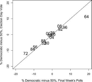
We begin at the end of the campaign timeline by seeing how well the final polls predict the vote. Figure 5.1 displays the Democratic vote as a function of the final week’s vote division in trial-heat polls. (Here and throughout this chapter, we measure the Democratic vote as the deviation from the 50 percent baseline.) From the figure we can see that the polls at the end of the campaign are a good predictor of the vote—the correlation between the two is a near-perfect 0.98. Still, we see considerable shrinkage of the lead between the final week’s polls and the vote. The largest gap between the final polls and the vote is in 1964, when the polls suggested something approaching a 70–30 spread in the vote percentage (+20 on the vote −50 scale) for Johnson over Goldwater, whereas the actual spread was only 61–39.
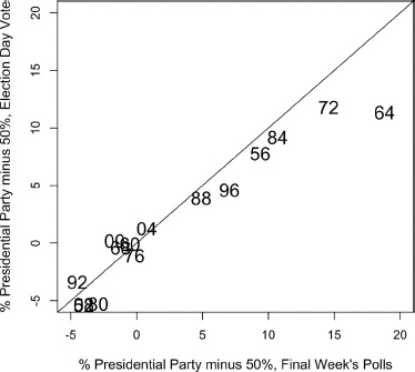
It is informative to flip the scales and repeat the vote-by-last-polls graph in terms of the incumbent presidential party vote instead of the Democratic vote, as in figure 5.2. This figure shows a clear tendency for the late polls to exaggerate the support for the presidential party candidate; that is, most of the observations are below the line of identity relating the polls and the vote. From the figure it also is clear that the underlying reason appears to be that leads shrink for whichever candidate is in the lead (usually the incumbent party candidate) rather than that voters trend specifically against the incumbent party candidate. When the final polls are close to 50–50, there is no evident inflation of incumbent party support in the polls.
Figure 5.1. Democratic party vote for president as a function of the democratic vote in the final campaign week, 1952–2008. The vote and poll vote divisions are reported as percentages of the two-party vote. The diagonal line represents a projection of the poll results on the y-axis. The closer a figure is to the line, the less the deviation of the vote from the final week’s vote division.
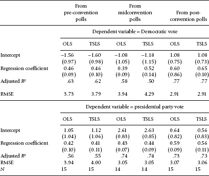
Table 5.1 extracts further statistical information regarding the vote-by-last-poll relationship. The details of the regression equation appear about the same whether we perform OLS, reliability correction, or TSLS and whether we predict the Democratic vote or the incumbent vote. In all instances, the coefficient for the polls is in the range of the mid-0.70s. All equations show a small negative intercept of about half a percentage point, suggesting that with the forecast of a close election, Democratic and incumbent party candidates perform slightly worse than projected. The deviations from zero are tiny and far from statistically significant, however. Thus, the final week’s presidential polls do not appear to be systematically biased.1
Of special interest are the reliability-corrected equations since these presumably correct for sampling error. Assuming perfect polls plus no intervening events between the last polls and Election Day, the RMSE in the reliability-corrected equations should approach zero. Instead, we see a standard error slightly greater than 1.0. We can ask, is this small but nonzero error a sign of inefficient polls? Or is it due to the quite plausible hypothesis that the “error” represents last-minute vote shifts between the polls and Election Day?
As a test, we can analyze the vote-by-last-polls equation separately for the seven earlier elections (1952–76) and the seven later elections (1984–2008). We omit the middle year, 1980, which is known to have considerable late movement in the final week’s polls. In the seven earlier elections, the N’s for the final week of polling are all below 5,000, with a median of 1,502. In the seven later elections, the N’s in the final week are all above 10,000, with a median of 22,944.2 Clearly the N’s are sufficiently large to imply little meaningful sampling error for the latter half of elections.
Figure 5.2. Incumbent presidential party vote as a function of the incumbent presidential party vote in the final campaign week, 1952–2008. The vote and poll vote divisions are reported as percentages of the two-party vote. The diagonal line represents a projection of the poll results on the y-axis. The closer a figure is to the line, the less the deviation of the vote from the final week’s vote division.
Table 5.1 Predicting the Election Day vote from the polls in the final campaign week, 1952–2008
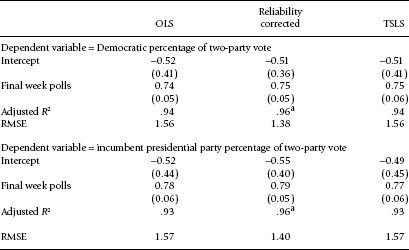
Note: The instruments for the TSLS equations are the post-convention vote divisions. Reliabilities are .988 for the percentage Democratic and .985 for the incumbent-party vote. Vote divisions in the polls and the vote are in terms of the percentage of the two-party vote minus 50. Standard errors are in parentheses.
a Estimated R2.
Our expectation is that if inefficient polling is responsible for the mild prediction error, we should see the greatest error for the early half of the series with smaller N. Instead, we find the largest errors for the later years. With reliability-corrected equations, the RMSE is 1.29 in the later years with heavy polling and only 1.07 in the earlier elections with sparser polling. Thus, the more recent elections with their increased wealth of late polling were slightly more difficult to predict from the late polls. This suggests that insufficient sample sizes are not the culprit behind the imperfect prediction. Rather, it seems that voter shifting is the source of late “error” and, since this error has increased over time in the face of more polling, that late electoral shifting has been on the increase over the span of our study.
Why do leads shrink during the final run-up to the election? One possibility is that the attenuation of leads in the final election verdict results from short-term influences that are tracked by the late polls but evaporate by Election Day. Estimation using TSLS provides a test. We ask: As instrumented by vote intentions measured eight weeks earlier, does the coefficient predicting the vote from the final polls increase? To the extent this is so, the OLS coefficient is depressed by inconsequential short-term influences on the polls that serve as the equivalent of measurement error. We consult the TSLS equations from table 5.1. The TSLS estimate is based on using the post-convention vote division as the instrument for the final polls. The idea, as in the TSLS analysis of polls in chapter 4, is to interpret the TSLS result as the estimate of the effect of the equilibrium portion of lagged vote intentions—here the intentions the week before the election in the trial-heat polls. Whereas the OLS coefficient reflects the equilibrium value of lagged vote intentions but is biased downward by short-term effects, the TSLS coefficient should represent only equilibrium effects.
The TSLS estimate predicting the actual vote from the presumed equilibrium value of the final week’s polls is virtually identical to the OLS estimate.3 Thus, even in terms of the equilibrium value, leads shrink between the final polls and the vote. This similarity of coefficients suggests that the presence of short-term campaign effects late in the campaign is not a major factor depressing the coefficient for the late polls.4
We can increase the parameter estimate for late polls by excluding the extreme 1964 case (when the Democratic landslide was even stronger in the final polls than on Election Day). This pushes the OLS coefficient (predicting the Democratic vote) all the way from 0.74 to 0.84. We can also recalculate the error correction adjustment without 1964. This nudges the coefficient to 0.86. We can conduct the TSLS version without 1964, and the coefficient advances to 0.88. As a final step, if we switch the prediction from the Democratic vote to the presidential party vote, again ignoring 1964, we gain just one more digit, with a coefficient of 0.89 (standard error = 0.07).
There is another possible influence on the coefficients that must be considered. By our construction, the preferences of undecided voters have been ignored. As the campaign evolves, the proportion of those who claim to be undecided shrinks. By modeling vote intentions as the two-party vote, we in effect assume that the undecideds’ split is identical to that of the decideds, an assumption that is certainly wrong (also see Campbell 2008a). Even if we allocate undecideds differently, however, the resulting coefficients reveal essentially the same pattern.5 Ultimately, then, the results imply an underdog effect, where the projected loser gains support at the very end of the race.
We are left with the simple possibility that most of the late switching goes to the disadvantaged party, though not by an amount that affects who ultimately wins. Conceivably, the shrinkage of leads could also be fueled by the polls’ failure to capture the full measure of support for the disadvantaged party. This could be a by-product of an often-hypothesized “spiral of silence” effect—by which those who support the likely loser feel sufficiently isolated or ashamed that they resist revealing their true preferences to interviewers (Noelle-Neumann 1984).
Chapter 7’s analysis of individual survey respondents provides clues that can be previewed here. Relatively few voters switch their vote choice late in the campaign. Relatively few undecided voters during the campaign end up voting, and those who do split close to 50–50. Moreover, there is no evidence that partisans “come home” to their party on Election Day (although this phenomenon occurs earlier in the campaign). Yet chapter 7 highlights one additional factor that explains why late leads shrink. Many survey respondents tell pollsters they will vote but then do not show up. These eventual no-shows tend to favor the winning candidate when interviewed before the election. Without the preferences of the no-shows in the actual vote count, the winning candidate’s lead in the polls flattens.
Knowing how well the final week’s polls predict the presidential vote provides an important end-of-campaign benchmark. Of course, the late trial-heat polls are silent about how the Election Day result comes into focus over the campaign. For this, we must assess the predictability of the vote from polls at earlier points in time. To this interesting topic we turn next.
While attention normally centers on the accuracy of the final polls, we give further attention to the earlier polls, which for many elections are found as early as 300 days before the election. We consider how well polls from different points in the campaign timeline predict the Election Day vote. The pattern of predictability furthers our understanding of the dynamics of the vote division throughout the long election campaign.
For this section, we measure vote margins in the polls not weekly as in the previous chapter and the previous section, but on a daily basis. We do this by simply interpolating the daily vote division from the polls in nearby days. When (as is often the case) a date has no poll, we assign the average of the vote division from the previous poll and the vote division from the next poll, weighting the two components by the closeness of their dates to the polls.6 For the last dates before the election, we score the vote division from the final poll.7
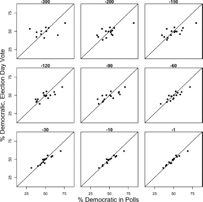
First consider the scatter plot of the relationship between poll results at various points of the campaign cycle and the actual vote. We illustrate with figure 5.3, expanding our database temporarily to include all dates within 300 days of the election. In the upper left-hand panel of the figure, using only elections in which polls are available 300 days before the election, we see that there is little relationship between these early polls and the actual vote. As we turn toward increasingly current polls, moving horizontally and then vertically through the figure, pattern emerges; simply, the later the polls, the greater the focus. That is, the points line up. The closer we get to the election, the more the polls tell us about the outcome.
Figure 5.3. Vote by vote division in polls at various dates from 300 days to one day before the election, 1952–2008. Daily polls are interpolated where missing.
Consider basic summary statistics focusing on the last 200 days, by which point we have polls in each election year. At 200 days before the election, reported poll results and the final vote differ quite a lot, by 6.4 points on average.8 At the 100-day mark, about the time of the national party conventions, the average difference between the polls and the ultimate vote is 4.9 points. By the very end of the campaign, the average difference is a mere 1.8 points.9 It thus is clear that the polls tell us more and more about the outcome as the campaign unfolds. This is not especially surprising, but it is a useful validation of conventional wisdom.10
To systematically examine the degree to which the polls at different dates predict the vote on Election Day, we generate a series of daily equations predicting the vote in the fifteen elections j during 1952–2008 from vote intentions in the polls at date T in the campaign timeline.
VOTEj = aT + bTVjT + ejT.
Using the statistics from these equations, we first present and interpret the dynamics of how the variance explained by the polls (R-squared) varies over the campaign timeline. Second, we present and interpret the changes in the regression coefficient (bt) as a function of the date.11
The R-squared statistic tells us how much of the variance of the dependent variable (here, the Election Day vote) is accounted for by the independent variable(s), here the date’s vote division in the polls. An important aspect of understanding the campaign timeline is the day-to-day trend in the R-squared predicting the final vote from the current polls. In the following section, we review some statistical theory regarding what the R-squared might tell us about the underlying time series. Readers without a strong statistical bent may prefer to skim or skip it, turning to the section that follows, which examines patterns in the data.
Theory
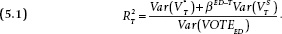
In terms of a formula,
In chapter 3, we posited that the vote division is a combination of an integrated series or random walk, V*, plus a short-term component VS. Statistically, these series components can be described for elections j as follows:

and

where the ujt and ejt error terms are the sources of  and
and  , respectively, following the terminology of chapter 3. For the moment, we conveniently assume that ujt and ejt are uncorrelated with each other and have constant variances over time.12 We also ignore the election eve compression of the vote variance, as the vote margin shrinks by about 25 percent from the final polls to the actual vote.13 With these assumptions and allowances, we can interpret the R-squared for any given campaign date T as follows:
The moving parts in the equation are all in the numerator. The model’s random walk assumption requires that the equilibrium variance Var( ) grows with time T. Meanwhile, the short-term component of the explained variance
  also grows larger as the campaign progresses. We are interested in the description of the potentially nonlinear slope describing the change in the R-squared predicting the vote as the campaign timeline increases from day to day, and what it might tell us about campaigns and voters. To develop some expectations, we see that the slope at time T is the first difference between the vote margin at time T and at T − 1:

and

By some algebra, the one-period change in the R-squared, therefore, is
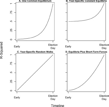
Let use consider some simple examples of how the net R-squared would look over time, based on equation 5.2. Clearly the explained variance should go up with time, but the functional form will depend on the proper model of the two components. Figure 5.4 displays four possible idealized models, varying as a function of the relative contribution of the two components.
Figure 5.4. Four models of the R-squared predicting the vote from polls at various dates over the campaign timeline. Each model assumes shocks of constant variance over the timeline.
The upper left-hand panel (A) presents the path of an R-squared from a baseline model in which the vote is a function only of short-term effects, with all campaigns in different years sharing one common equilibrium value for V*. By this model, the vote division in different years at the same time T during the campaign reflects variation around a common mean. In the long run—if campaigns were extended indefinitely—the early vote division would provide no information regarding the vote at the end of the process. This is because any difference between early polls and the common mean would decay by Election Day, leaving V* as the expectation in each year. Late polls would provide information, however, as they reflect campaign effects that do not fully decay by Election Day. The result in terms of R-squared is the nonlinear temporal pattern shown in panel A, as the R-squared starts at zero on its path toward 1.0.
Next, consider panel B in the upper-right corner of figure 5.4, which shows the path of the R-squared if the vote is a function of both . and . Here, the equilibrium term varies by year j but does not move over the campaign timeline. This model represents a set of stationary series varying around different yearly means, as discussed in chapter 3 (see fig. 3.2). The result in terms of R-squared bears the form of the nonlinear pattern shown in panel A, reflecting late-arriving campaign effects. But here in panel B, reading backward in time from Election Day, the curve trends toward a nonzero constant. This constant represents the contribution of the equilibrium values  , which do not change during campaigns.
Next, consider panel C, which shows the results if campaign vote divisions were the result solely of a random walk over the campaign timeline. Here, the R-squared evolves linearly over time with the accumulation of shocks with no decay. Of course, the linearity is a function of the assumption of shocks with constant variance over time. If shocks are larger at some points in the campaign timeline, the slope of the R-squared regression line would be steeper for those intervals.
Finally, panel D presents the R-squared panel expected with both a random walk and stationary component. Here, the long-term component drives the results, as short-term variation around equilibrium is relevant for the actual vote only when it occurs late in the campaign.14 The R-squaredby-time function would take a form that effectively combines the curves in panels A and C. As shown in panel D, there would be a linear trend that curves upward toward the end under the influence of late short-term forces, as late events have most sway on the vote.15
Which, if any, of these graphs should we expect as an accurate portrayal of the R-squared? Our hypothesized model has both a long- and short-term component to the poll margins, so that would seem to push us to model D. We must, however, be open to campaign shocks of uneven impact throughout the campaign. With the reality of a net decline in the cross-sectional variance of the vote division and the assumption of a random walk component, it may be that the short-term shocks do decline in magnitude over time. Suppose this is true, and Var( ) declines toward zero. Suppose also that the rate of change of the R-squared also changes as a function of declining permanent ut shocks.
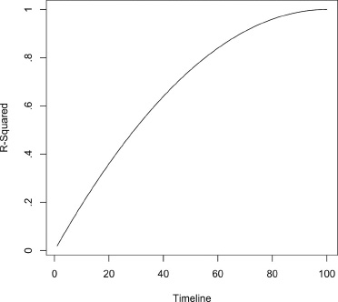
Figure 5.5 presents one example where the variance of the short-term forces () declines linearly from time 1 to zero at time ED, while the ut shock variance declines in such a fashion that it becomes inconsequential by Election Day. Given this input, figure 5.5 shows a rising R-squared with a slope that declines with time.
Figure 5.5. Model of R-squared where the vote is governed by year-specific random walks over the campaign timeline, with the variance of shocks declining linearly over the timeline, ending at zero on Election Day.
Which (if any) model provides a fit with the actual change in the adjusted R-squared over the campaign timeline? Let us see what the data reveal.
How does the R-squared change predicting the vote from the polls change over the course of the campaign season? When comparing the R-squareds at different points in the campaign timeline, it is crucial to compare regressions with the identical set of years. If we were to vary the years from one date to the next, the R-squared would vary with the variance of the vote. Including landslide Republican and Democratic years would expand the variance and the R-squared; to concentrate on close elections would have the opposite result. Fortunately, trial-heat polls were already in place by January in 11 of our 15 presidential election years. We start with date ED-300, that is, 300 days before Election Day. For each date in this sequence, we regress the vote on the polls, interpolating for the many date-year combinations for which actual polls were not available. The four election campaigns we must omit for this exercise are 1952, 1968, 1972, and 1976. In January of these years, the pollsters evidently saw little chance that Stevenson (1952), Nixon (1968), McGovern (1972), or Carter (1976) would be party standard-bearers, even though two from this list went on to victory in November.
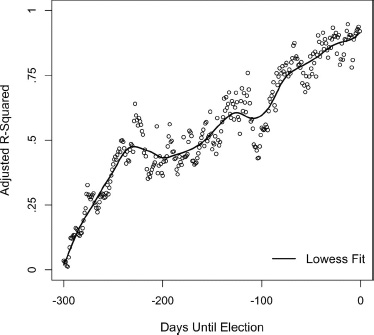
Figure 5.6 presents the result, using the statistically appropriate adjusted R-squared, which is the more conservative estimate of fit that takes into account the sample size. Much like the hypothetical graph in figure 5.5, the adjusted R-squared starts at near zero, increases rapidly, and gradually levels off on its march toward 1.00. Judging from the modesty of the increments, it would seem that the battle lines shift very little during the late campaign. In terms of our model, election shocks would start big and end up small. During the first 100 days of the election year, there apparently is a lot of learning about the campaign. Permanent shocks to the vote are increasing, while the seemingly large short-term effects (evident from the large cross-sectional variance of the vote) begin to burn off.
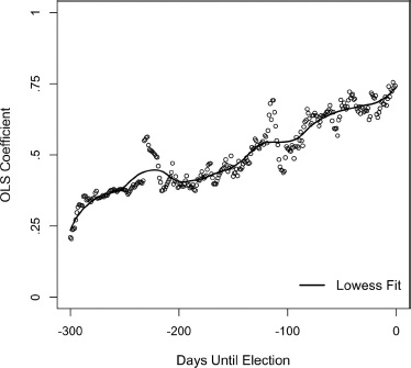
Figure 5.6. Adjusted R-squared predicting the Democratic vote from the Democratic vote division in the polls, by the date in the campaign timeline starting 300 days before Election Day. For eleven elections with polls going back 300 days, 1956–1964, 1980–2008. Daily polls are interpolated where missing. Lowess fit is with a bandwidth of .20.
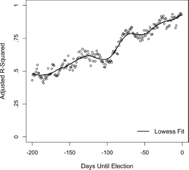
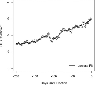
Figure 5.7. Adjusted R-squared predicting the Democratic vote from the Democratic vote division in the polls, by the date in the campaign timeline starting 200 days before Election Day. For fifteen elections, 1952–2008. Daily polls are interpolated where missing. Lowess fit is with a bandwidth of .20.
Figure 5.7 displays the cross-sectional R-squared from regressing the vote division on the poll division for each date starting 200 days before the election, when we have polls in all fifteen election years. Focusing on the final 200 days highlights a substantial growth in the R-squared in midsummer, where another bout of voter learning occurs. The figure reveals an interesting pattern: polls from 100 to 200 days before Election Day increase gradually in prediction accuracy. They also contain important information, as the R-squared hovers between 0.50 to 0.60. In effect, we have half the Election Day story six months before the election and gain relatively little in the ensuing three months. The largest improvement in predictability comes from about 100 days out to about 70 days out (typically the convention period), as a midsummer spurt. Thereafter the slope of the R-squared flattens out and increases only incrementally. That is, the polls add an equal amount from day to day, on average, and peak at the end of the campaign, where the R-squared for the vote-on polls regression reaches a healthy .93.
Figures 5.6 and 5.7 teach us quite a lot. At the start of the election year, polls are taken but they are virtually meaningless for election forecasting purposes. In January of election year (measured here by polls on day ED-300), the polls involving the eventual major-party presidential candidates can explain a mere 4 percent of the variance in the ultimate vote margin. Still, a candidate would rather be ahead than behind at the early date. The leader in January won the election in eight of the eleven contests for which we have polls at that early date in the campaign timeline.
By April, the primary season is under way and, in most recent years, practically over. The candidates running paired in our trial-heats are no longer hypothetical choices. Rather, they are heavy if not prohibitive favorites to win their nominations. And by this time, the trial-heat polls between the eventual candidates can account for 43 percent of the variance in the vote. Further learning slows as the conventions approach. From day ED-200 to ED-100—approximately mid-April to mid-July—predictability from the polls improves by an additional 16 percent.
As the campaign moves into the summertime phase, campaign shocks grow with a lasting effect on the outcome. We know this because the predictability of the election outcome increases strongly through the summer months. From 100 days to about 70 days before the election, the adjusted R-squared jumps 22 points. As we will see, this is a function of the party conventions held during this period. By date ED-70 (late August), the convention spurt has ended. From this point until Election Day, the R-squared increases by its final 12 percentage points. The fall campaign leaves an imprint on the vote, but no more than that during the April-to-July interregnum, and certainly less than during the primary season or the convention period. By the beginning of the fall general election campaign, the result is almost hardened in place.16
Our next set of clues are the regression coefficients over the campaign timeline—the regression coefficients predicting the vote from the polls over the final 200 days of the campaign. Below we show the series of regression coefficients predicting the vote from the polls, for each date going back 300 days (for eleven years) or 200 days (for all fifteen years) from the election. As with our discussion of the R-squareds, we first present some theory. The less statistically inclined can skim or else skip to the data section just below.
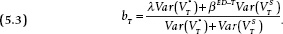
The observed bT represents the expected proportion of the observed vote margin that will survive to Election Day. But what about the equilibrium portion of the vote division? Let us define λT as the unobserved parameter representing the effect of —the equilibrium portion of the vote division on the vote. The estimate bT is not λT but rather a complicated compound incorporating the combined and effects (λT and βED−T). Specifically,
To understand how bT varies with time, let us mentally divide the timeline into two segments. In the early segment, the short-term shocks do not last to Election Day, that is, βED−T approaches 0, leaving only the first component of the numerator of equation 5.3. But the short-term component is present in the denominator, functioning as if it is measurement error in the calibration of the equilibrium component. During this period, the bT estimate of λ is biased downward in proportion to the size of the short-term variance in relation to the equilibrium variance . In the absence of short-term shocks, that is, where  , equation 5.3 simplifies to the equilibrium effect (i.e., bT = λT for all segments of the timeline).
Now consider the later segment of the timeline. Here the short-term component matters and the second term of the numerator of equation 5.3 is greater than 0. In contrast with the first segment, therefore, the b coefficient will surge in size. The surge will depend on the extent to which the late, short-term variance () affects the vote.
Figures 5.8 and 5.9 present the bT coefficients over the campaign timeline. The size of bT reveals, as an expectation, the proportion of the time T lead that will survive until Election Day. The central fact that stands out from figures 5.8 and 5.9 is the low but growing magnitude of the coefficients. The expectation is that poll margins at any point in time will shrink by Election Day, and the farther from the election, the greater the shrinkage. Leads in January (300 days out), for instance, will shrink (as an expectation) up to 80 percent by Election Day (bT about 0.20). At about 100 days out (midsummer) the shrinkage level is about half. And as we saw earlier, even the poll margins of election eve trim by 25 percent on Election Day.
Figure 5.8. OLS regression coefficients predicting the democratic vote from the Democratic vote division in the polls, by date in the campaign timeline, starting 300 days before Election Day. For eleven elections with polls going back 300 days, 1956–1964, 1980–2008. Daily polls are interpolated where missing. Lowess fit is with a bandwidth of .20.
Taking a close look at the full scan of 300 days (fig. 5.8), we observe a curve whose highlights mimic the R-squared curve of figure 5.6. The bT starts out as low as 0.20 but quickly zooms up during the early months of the campaign. To observe the continued rise toward 0.75, we turn to the 200-day picture of figure 5.9. The trend appears fairly linear. Yet we can discern two more periods of steep growth in an otherwise wiggly line with a linear trend. One such period is the convention season around midsummer. The second is at the very end of the campaign. Whereas short-term campaign effects generally dissipate before the election, those that arise near the campaign’s end can and do affect the vote.
Figure 5.9. OLS regression coefficients predicting the Democratic vote from Democratic vote division in the polls, by date in the campaign timeline starting 200 days before Election Day. For fifteen elections, 1952–2008. Daily polls are interpolated where missing. Lowess fit is with a bandwidth of .20.
What can we add regarding our understanding of the dynamics of vote intentions from figures 5.8 and 5.9? If we assume a constant λ—the effect of the equilibrium component of preferences—of about .75, the growth of bT would be a signal of an ever-decreasing shrinkage of the variance of the short-term forces. But the λ term could also be changing. The equilibrium component could be an integrated series as we have posited, yet still show further compressions of its metric similar to that from the late polls to the vote. One such compression we saw from chapter 4 occurs at conventions time, when the TSLS regression of the post-conventions vote division on the pre-conventions vote division is about 0.70 instead of approaching 1.00. Can we do more with our slopes predicting the vote from the polls to estimate the λ parameter?
We can obtain some purchase by once again applying TSLS. In chapter 4 we ran several TSLS regressions predicting the vote division from the lagged vote division, using the vote division lagged 9 weeks. The idea is that vote intentions at lag-9 comprise a good instrument for the lag-1 long-term component  , as it is relatively free of the short-term forces present at lag-1, 8 weeks later. We can use the equivalent instrumentation—the interpolated vote division at lag-8 as an instrument for vote intentions at time T in a regression predicting the vote from at time T.17
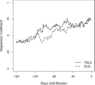
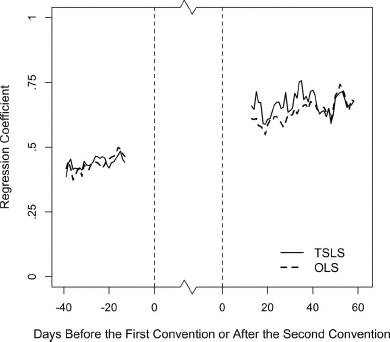
We present the results graphically in figure 5.10. For the final 160 days of the campaigns, the figure compares the daily slopes from our OLS analysis (from fig. 5.9) with the TSLS estimates.18 Both early in this segment of the election cycle and toward the very end, we see the two series tracking each other. In the middle—the convention season—the two series diverge with the TSLS estimate larger. This gap continues and actually widens some, and then slowly closes after the convention season is over.
The TSLS estimate is intended as an estimate of how much of the long-term component (λT), of the vote division persists to Election Day. We see it hold remarkably steady at about 0.65 from about 100 days out until the final week. The implication is that, for this time period, if we knew which portion of the poll results is the long-term component rather than short-term effects or measurement error, about 65 percent of the lead would hold, as an expectation, until Election Day. The gap between the TSLS estimates and their OLS counterparts is evidence of short-term forces. Where OLS underestimates λT, the culprit would be short-term forces acting as the equivalent of measurement error dampening the observed statistical estimate.
Figure 5.10. OLS and TSLS regression coefficients predicting the Democratic vote from the Democratic vote division in the polls, by the date in the campaign timeline starting 160 days before Election Day. For fifteen elections, 1952–2008. Daily polls are interpolated where missing.
It seems logical for strong short-term forces to be present during the convention season and for a little while thereafter, as the convention bounces wind down. It is plausible that there would be no appreciable short-term effects at campaign’s end (when the OLS–TSLS gap closes). It is somewhat of a surprise, though, to find evidence that short-term forces are virtually absent in the period leading up to the convention. We return to this puzzle in the next section, where our analysis fixes on the convention period and how it compares to times immediately before and after.
In chapter 4’s analysis of the vote division over time, we saw that the conventions were a period of interruption in an otherwise stable pattern in which each year’s vote division holds fairly steady week by week. Here we examine the convention effect on the Election Day vote. Following our procedure for examining convention effects in chapter 4, this section models the vote as a function of the incumbent party vote rather than the Democratic vote. And we measure time not in terms of days before the election but rather as days before and after the two major-party conventions.
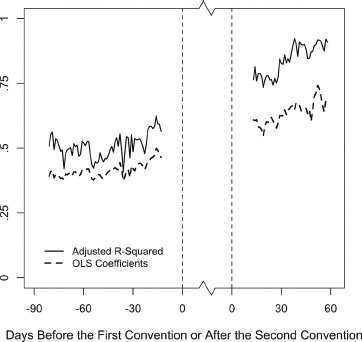
Our first step is to repeat the analysis of adjusted R-squareds and regression slopes over time, where the timeline is relative to the conventions. Figure 5.11 shows the results of the OLS analysis. The figure should not surprise. We see gradual increases in the observed R-squareds and b slopes as the timeline progresses. The coefficients are well behaved as mildly sloping linear lines, with an evident break during the convention period.19 We leave a big window on each side of the convention period where we present no coefficients, because during these intervals the interpolated estimates are for some years “contaminated” by heavy weighting of data from surveys within the convention window. We include only dates for which estimates can be obtained using data from all fifteen elections.
Figure 5.11. Adjusted R-squared and OLS regression slopes predicting the vote by date of the vote division in the campaign timeline relative to party conventions, 1952–2008. Negative dates indicate the number of days before the first convention, from −82 to +14. Positive dates are the number of days after the second convention, from +14 to +59. The date scale compresses the time gap between −14 and +14. The average period from the start of the first convention to the end of the second convention is 31 days. Daily polls are interpolated where missing.
For greater understanding, we turn to TSLS estimates of the regression slopes. Here, the goal is to obtain estimates of the equilibrium effects (λT) free of the influence of the measurement error due to short-term forces. Figure 5.12 shows the results—a comparison of the OLS estimates (from fig. 5.11) with TSLS estimates for dates pre- and post-convention. The TSLS estimates are quite level, both before and after the conventions, but at different heights. After the conventions, the TSLS slopes average 0.67, as if about two-thirds of the presumed fundamentals from a date of the late campaign carry over to Election Day. This average is close to the ceiling of 0.75 observed at election eve. Before the conventions, the average slope is 0.46, or roughly two-thirds of the post-convention slope of 0.67, which mirrors the slope of about 0.67 (from chap. 4) predicting the post-convention vote division from pre-convention values.20
Figure 5.12. OLS and TSLS regression coefficients predicting the Democratic vote from the Democratic vote division in the polls, by the date in the campaign timeline relative to the party conventions. Negative dates are the number of days before the first convention, from −40 to 14. Positive dates are the number of days after the second convention, from +14 to +59. The date scale compresses the time between −14 and +14. The average period from the start of the first convention to the end of the second convention is 31 days.
In figure 5.12, the gap between the OLS and TSLS estimates should serve as a rough estimate of the degree of short-term forces biasing the OLS estimates at different time points relative to the conventions. These results help clarify the patterns shown in figure 5.10. Both before and after the conventions, the OLS slopes virtually match the TSLS slopes. Prior to the conventions, the two sets of slopes each average 0.46. Following the conventions we see a tiny OLS–TSLS gap, although the discussion that follows suggests it is probably not meaningful. Whereas the average slope post-convention (14 to 59 days after the second convention adjourned) was 0.67 estimated using TSLS, it is 0.64 estimated using OLS.
The similarities between the two sets of slopes offer some convenience. If short-term sources of variation in vote intentions do not matter much, then the OLS estimates should be good enough to estimate the relationship between the results of the polls and the eventual vote. The stable slopes within the pre- and post-convention time frames suggest that most influences on vote intentions during these periods leave permanent imprints that survive to Election Day.
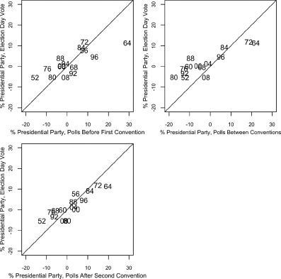
At this point, we can gain a firmer foothold by turning to the relationship between what the polls show during the convention season and the Election Day vote. Figure 5.13 shows scatterplots, where the vote is measured as support for the presidential party. The statistical details are in table 5.2. The table shows the predictions of the vote before, between, and after the conventions—both in terms of the support for the Democratic candidate and for the incumbent presidential party.
Figure 5.13. Incumbent party vote by incumbent party vote division in the polls before, between, and after the major party conventions, 1952–2008. (There is no midconvention reading for 1956.) The diagonal lines represent projections of the poll results on the y-axis. The closer a number to the line, the less the deviation of the vote from the final week’s vote division.
Table 5.2 Predicting the Election Day vote from polls before, during, and after the major party conventions
Note: The instrument for the TSLS analyses is the vote division in early April, week ED-200. The pre-convention polls are the weekly polls for the week ending the Monday before the first convention. The post-convention polls are the weekly polls for the week beginning the second Tuesday after the second convention. There is no midconvention reading for 1956. Vote divisions in the polls and the vote are in terms of the percentage of the two-party vote minus 50. Standard errors are in parentheses.
The upper-left panel of figure 5.13 shows the in-party vote as a function of pre-convention vote intentions, our benchmark measure from chapter 4. Note the shallow slope. The stronger the in-party showing in the pre-convention polls, the greater will be its decline by Election Day. The pre-convention polls correlate at a modest 0.77 with the final vote.
The upper-right panel shows the in-party vote as a function of the between-conventions vote division. The prediction tightens, as the correlation zooms from 0.77 (panel 1) to 0.87 (panel 2) in just a few short weeks. This shows that the first (out-party) convention produces real learning on the part of the voters of the sort that survives to Election Day.21 Still, the out-party gain is usually offset by the impact of the second convention, as the in-party usually outperforms its between-conventions polls on Election Day (see the positive intercept in table 5.2).
The bottom panel of figure 5.13 shows the in-party vote as a function of the post-convention polls, measured the second week after the final convention as in chapter 4. The slope now steepens as the variance of the polls compresses from the between-conventions to post-convention periods. And the inflation of the out-party vote evident between the convention vanishes. (In table 5.2, the intercept returns to near zero.) The polls-vote correlation grows no further between the periods.22
Thus, consistent with all expectations, the vote division first shifts toward the out-party after its convention and then back toward the in-party after its event. In effect, the conventions produce substantial bounces. It should be emphasized that the net convention effect is more of a bump than a bounce for the party that walks away from the conventions with the net vote advantage. We saw in chapter 4 that the party that increased its vote support from pre- to post-conventions on average gains 5.2 percent of the vote, a margin that persisted to the final polls. Here, we note that this gain persists and actually increases slightly (to 5.5 percent) by Election Day.23 When a candidate leaves the convention season with a net gain in the polls, the gain persists not only in subsequent polls (as shown in chap. 4). It persists to Election Day.
This chapter has documented the relationship between the vote division throughout the election year and the Election Day vote. At the beginning of the year, vote intentions tell us little about the final outcome. Rapid learning takes place during the presidential primary season and, by the end of the nomination process, the electorate’s preferences begin to take shape. They still are only half-formed at this point in time. The conventions stimulate further learning, and preferences are largely crystallized entering the general election campaign. Surprisingly little changes from the conventions to the final week of the campaign. At that point we observe the last minute shifts from trial-heat polls to the vote, described at the outset of this chapter.
Along the way of our analysis, we have distinguished between the long-term component of the vote—the permanent accumulation of electoral shocks—and the ephemeral short-term variation around it. The latter may be of little significance except at the very end of the campaign. The former clearly evolves over the election year.
It is striking that in early January (300 days until the election), the reported vote intentions in trial-heat polls vary quite a bit from one election year to another, yet do a poor job of predicting the Election Day vote. On the basis of our analysis, the events that influence aggregate electoral preferences before the election year even begins must have no real impact on the Election Day result. Since they ultimately do not predict the vote, they are short-lived, and do not stand the test of time.
Meanwhile, as the election year begins, the fundamental forces of the campaign are beginning to take shape. Left to be discussed is the nature of the fundamental forces that drive this long-term component of the vote in each presidential election. That is the focus of the next chapter.