Previous chapters have dealt solely with the aggregate vote intentions over the campaign timeline. In this chapter we zoom in to focus our microscope on individual voters. We seek to assess the degree of vote choice stability at the individual level that underlies the net aggregate stability we have observed. How stable are the individual vote decisions that comprise the aggregate change? And who changes? Further, we seek to understand further how the structure of vote choice varies across the campaign timeline. Are different voter motivations activated at different times? Can we gain further understanding of the changes in the cross-sectional aggregate vote intentions over the campaign timeline?
The wealth of available survey data from sources such as the Inter-University Consortium for Political and Social Research (ICPSR) and from the Roper Center’s iPoll presents a host of opportunities. We focus first on the American National Election Studies (ANES) presidential polls available from ICPSR. For each presidential year included in our analysis, the ANES interviews a panel of respondents both before and after the election. We assess the differences between the pre-election vote intentions of the panelists and their post-election reports of their vote decisions between 1952 and 2008.
The ANES pre-election interviews are concentrated in September and October of the election years. We also model individual voters from Gallup polls at or near the four key time points of the campaign identified in earlier chapters—April (around ED-200), just before the first national party convention, a week after the second convention, and the final poll of the election season. This represents voters in 4 surveys × 15 years for 60 polls altogether. From these cross-sectional surveys we are interested particularly in the growth of voters’ reliance on their personal fundamentals. That is, we want to see whether and how the structuring effects of partisanship and demographic variables change over the campaign timeline.
Observers often write about voters as if they are very malleable and subject to persuasion from the latest political information that reaches their attention. Yet, we have seen that in the aggregate (and when adjusting for sampling error), vote intentions from one period to the next in a campaign tend to be very stable. Suggestive though this is, the aggregate stability does not necessarily require a similar degree of stability among individual voters. For instance, suppose that over one week the Democratic candidate gains 2 percent of the vote (which would be a major change in the scale of things). This net change of two percentage points could come in many combinations of Republican voters shifting to the Democratic candidate and some Democratic voters shifting to the Republican candidate. It could result from a mere 2 percent of the voters switching from Republican to Democratic, with none doing the reverse. But the change could also be due to 10 percent switching from Democrat to Republican, offset partially by 8 percent moving against the grain from Democrat to Republican. The key is that the Democratic gain would need to be two percentage points higher than the Republican gain in order to add up to a net 2 percent.1
Given the strong stability of the aggregate vote division, one might expect that the most plausible scenario at the individual level would be a degree of turnover at the individual level near the low end of what is theoretically possible rather than a continual churning of voter preferences back and forth. As we will see, this expectation is largely correct.
A useful starting point for understanding the stability of voter preferences within campaigns is to ask, How stable are presidential vote choices between elections—that is, from one election to the next? Over the fifteen elections of our study, the average absolute change in the two-party vote for president (compared to four years before) is 6.7 percentage points. In electoral politics, this is a large amount of change. So how much do individual voters change from one election to the next to account for the observed electoral change?
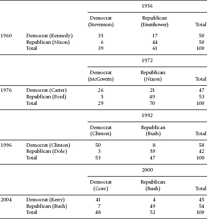
The American National Election Studies (ANES) has conducted four separate panel studies in which the same voters were asked their presidential vote following two successive elections. These panels were over the periods 1956–60, 1973–76, 1992–96, and 2000–2004. Table 7.1 displays the 2 × 2 turnover tables for these elections—that is, the Republican or Democratic vote choices in the second election as a function of the Republican or Democratic choices in the first election.2
Table 7.1 Reported vote choice by major party voters in successive elections in four ANES panels
Source: Data are from ANES panel data sets.
Note: Panel percentages do not necessarily represent those of the voting population. Data are weighted where appropriate.
In the two most recent panels (1992–96 and 2000–2004), the net vote division changed little between the first and second elections, either in the official verdict or among the ANES panel. Table 7.1 shows that this was also true at the individual level. From the first Clinton victory to the next (1992 and 1996) and from the first G. W. Bush victory to the next (2000 and 2004), about nine out of ten voters who cast a major-party ballot both times voted for the same party’s presidential candidate both times.
The two earlier panels each involved a larger electoral shift—from Nixon’s landslide in 1972 to Carter’s victory over Ford in 1976 and from Eisenhower’s landslide victory to Democrat John Kennedy’s close victory over Nixon in 1960. Even in these examples of major electoral change, only a few individuals (among those voting both times) created the difference. The 1972-to-1976 change among the ANES panelists who voted in both elections was an 18-point Democratic gain, split as 21 percent Nixon voters switching to Carter and a mere 3 percent switching against the grain from McGovern to Ford. The 1956-to-1960 shift was 11 points, with 17 percent shifting from Eisenhower to Kennedy. A larger than usual 6 percent shifted against the grain from Stevenson to Nixon, perhaps in a rejection of Kennedy’s Catholicism.
These examples ignore other aspects of electoral change. Consider, for example, panelists who report voting for a major-party candidate in one election but abstaining or casting a minor party ballot in the other. In the ANES panels, these respondents typically split their major-party votes about the same as those who cast major-party vote both times. Another source of change is by voters not in the panel: the differential between voters exiting the electorate in the first election and newly eligible voters in the second election. For example, one informed estimate of Obama’s victory in 2008 is that it could not have been done without the newly enfranchised young voters and the turnout surge among African Americans (Ansolabehere and Stewart 2009). In other words, among established voters who had voted in 2004, Obama probably would have lost. For all the turmoil and change between 2004 and 2008, including the collapse of both Bush’s popularity and the economy, very few voters changed their mind. The election of 2008 was decided by an infusion of fresh voters into the electorate.
The small amount of turnover of individual votes from one election to the next provides something of a ceiling regarding how much change we might find during a campaign. As we have seen, in the absence of a strong net swing of the vote, typically only about 10 percent will shift the party of their presidential vote. Common sense suggests even less shifting occurs within the context of a single presidential campaign. That is what we find.
In each presidential year since 1952, the American National Election Studies conducts both a pre- and a post-election interview for its panel of respondents. This makes it possible to assess the degree of turnover of choice from the campaign season to Election Day. Because pre-election interviews are scattered across the final 60 or so of the campaign, the date of the initial interview provides further leverage. We can assess not only the degree to which the respondent’s vote departs from the respondent’s stance during the campaign, but also the degree to which the change is a function of the date in the campaign timeline.3
We measure consistency of pre-election intention and post-election choice as follows. The cases consist of respondents who both expressed a major-party preference with their pre-election vote intention and then post-election said that they had cast a major-party vote on Election Day. Among these respondents, we simply counted the percentage of the cases in which their Election Day vote was for the same party/candidate as their pre-election vote intention expressed in September or October.
The answer is that 95 percent of ANES respondents maintained their pre-election position on Election Day. For caution, we should consider that it is possible that the panel interview format encourages an artificial degree of consistency. First, the respondents who continue in a panel might be somewhat more politically attentive—and therefore perhaps more consistent in their choice—than citizens at large. Second, and perhaps more importantly, the initial pre-election interview—in the home, lasting more than an hour—could sensitize people to defend their initial choice or see it as socially desirable to be consistent. Evidence exists, for instance, that ANES panel participation encourages respondents to vote at a higher than average rate (Burden 2003). Still, even if slightly inflated, the finding that 1 in 20 voters who express an intention in the pre-election ANES survey changes his or her choice in November is a sign that the vast majority of voters maintain the same vote choice over the campaign.
This result affirms that the small changes in the aggregate vote described in earlier chapters are a function of rare shifts by individual voters rather than a continual churning of preferences in response to campaign events. We next investigate the types of voters who shift their candidate preference from the campaign to Election Day.
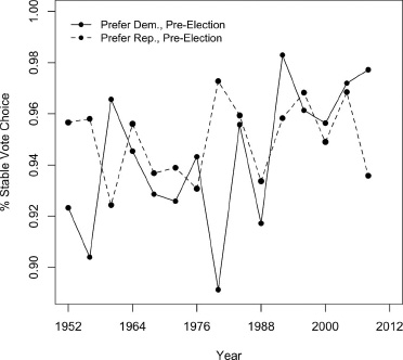
Figure 7.1 documents the degree of shifting, campaign to Election Day, by year and by the voter’s initial (campaign season) candidate preference. A slight trend can be discerned in that choices have been getting more stable over the years. Thus, we have a paradox of sorts. Voters have become increasingly exposed to presidential campaigns on broadcast and cable television, and now the Internet. Yet at the same time the effectiveness of campaigns in terms of changing voters’ minds seems to be on the decline. Although this finding is surprising given the greater access to campaign information, it is precisely what we would expect given increasing party structuring of the vote (Bartels 2000).
Figure 7.1. Stability of vote choice from pre-election interview to Election Day, by initial party choice, 1952–2008. Source: American National Election Studies.
Also of interest is the possibility of asymmetry in the degree to which initial Democrats and initial Republicans (in terms of vote intention) stick with their choice on Election Day. Whether Republican conversions or Democratic conversions are more prominent varies from year to year with no clear pattern. The strongest party difference is for 1980, when ANES respondents (like the nation) shifted from Carter to Reagan as the campaign progressed. The 2008 election provides a lesser instance, where the conversion rates favored Obama over McCain.
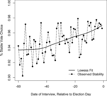
Further inference about vote choice stability can be learned from the degree to which rates of conversion vary with the time differential from the campaign interview to Election Day. Figure 7.2 presents the ANES respondents’ stability as a function of date of initial interview, pooling over all fifteen election years. The dashed line represents the observed daily observations. The daily observations show an erratic pattern if observed “day to day.” The curved line in the graph represents the smoothed (lowess) curve designed to provide the best fit to the data.4 The curve shows a steady increase in pre-election to vote stability, rising from .93 at 60 days before the election to .97 on Election Day.
Thus, as one would expect, stability rises as Election Day approaches. The shift is within a very small range, however. When summed over many elections, the data suggest that about 3 of 100 who hold a preference the day before the election switch on Election Day. The switch over the final 60 days is little over twice as high, about 7 in 100. A reasonable—simple but rough—inference is that from date ED-60 to date ED-1, only about 4 percent of voters switch their preferences. In other words, the data suggest about as much individual-level volatility over the fall campaign as on Election Day itself.5
Figure 7.2. Stability of vote choice from pre-election interview to Election Day, by date of interview, pooling observations, 1952–2008. Source: American National Election Studies.
If one looks to predict vote switching, the level of political knowledge is at the forefront. As is well known, informed voters tend to be resistant to campaign information because their knowledge leads them to form firm choices. It is the least informed who are more likely to switch during campaigns or from one election to the next (Converse 1962; Zaller 1992, 2004).
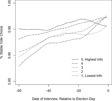
Figure 7.4 examines stability of vote choice as a function of both time and information level, keeping in mind that ANES data are available only for, at most, the last 60 days of the campaign. Information or knowledge level is measured using John Zaller’s composite index of political knowledge for the years 1952–2004.6 The index is standardized so that the mean is approximately 0 and the standard deviation is about 1.0 for each election year. Here, we divide the index into five categories from highest to lowest as follows, in terms of standard deviation units (SDUs):
5 = +1.5 SDUs or higher;
4 = +.5 to 1.5 SDUs;
3 = −0.5 to +0.5 SDUs;
2 = −1.5 to −0.5 SDUs;
1 = less than −1.5 SDUs.
For the most part, figure 7.3 shows precisely the pattern expected by theory. When measured shortly before the election, all information groups show high degrees of stability in the .97 range and are statistically indistinguishable. The most-informed groups, however, are consistent across the 60 days of the timeline, while the least-informed show a fairly steep lowess curve. Election Day votes by informed respondents are consistent with their choice 60 days earlier about 94 percent of the time. Informed voters have largely made up their mind before the fall campaign. But the least-informed fifth of the electorate’s votes are consistent with their early campaign preference only about 86 percent of the time.
Figure 7.3. Stability of vote choice from pre-election interview to Election Day, by date of pre-election interview and Zaller’s index of political knowledge level (lowess fit), pooling ANES observations, 1952–2004.
Overall, the impact of information is sufficiently strong to compete with the date of interview as a predictor of the stability of the vote choice. When both linear date and the original Zaller information index are included as independent variables in a probit equation predicting stability or change, they are both highly significant (z = 4.9 and 4.7, respectively). A voter’s level of information is about as good a predictor of whether she will defect from her pre-election choice as the date of the pre-election choice.7
The results of figure 7.3 serve to reinforce the conventional view that electoral change during the campaign arises mainly from the least sophisticated voters. Informed voters, particularly those in the two top information categories, were quite resistant to change. Among the relatively informed, only about 1 in 20 voters switches their candidate preference over the fall campaign. The less informed, while still highly stable, provided the most change. About 1 in 7 among the least informed voters will switch from the campaign interview to the vote. It is these voters to whom campaign appeals are most successful.
To a growing number of scholars, the primary function of election campaigns is to deliver the so-called fundamentals of the election. Recall from chapter 1 that we distinguish between external and internal fundamentals. Chapter 6 explored the external fundamentals—the political and economic conditions that structure candidate appraisals. These external fundamentals not only include the degree of economic prosperity but other aspects of performance and policy as well, including the policies and policy proposals of presidents and presidential candidates. Here we consider the “internal” fundamentals, whereby the campaign activates the political predispositions of voters.
As discussed in chapter 1, the literature on campaign effects finds considerable support for the campaign as causing voters to consult their predispositions. Finkel (1993) shows that much of the change in presidential vote preference during the 1980 campaign was due to “activation” of political predispositions, with voters bringing their candidate preferences in line with their preexisting partisan and racial identities. Relatedly, Gelman and King’s (1993) detailed analysis of 1988 polls shows that the effects of various demographic variables on presidential vote preferences increased over the campaign. A similar study of Pew polls during the 2008 campaign found partisan and demographic factors increasing in importance (Erikson, Panagopoulos, and Wlezien 2010). In short, campaigns appear to “enlighten” voters about which candidate(s) best represent their interests.
Over the campaign, voter preferences crystallize. Early on, when most voters are not thinking of presidential politics, these preferences are largely unformed. When interviewed, some will say they are undecided. They also may express weak preferences. Some may flirt with candidates from the other party. As the campaign unfolds, voters increasingly support the candidate of their preferred party. Voters’ preferences also increasingly reflect their true “interests” as reflected in their demographic characteristics. This crystallization may be driven by a number of mechanisms. Following Gelman and King (1993), campaigns help voters to learn which candidate best represent their interests, and typically this leads them back to their partisan attachments. Finkel (1993) argues that voters learn that the candidates really are partisans, representing Democratic and Republican positions and interests. Alvarez (1997) maintains that uncertainty about candidates’ issue positions is reduced as campaigns unfold. Yet another possibility is that campaigns lead voters to perceive events using their partisan screens, leading them to see candidates of their party more favorably (and increase the intensity of their support) as the campaign unfolds. The latter mechanism is implied by The American Voter (Campbell et al. 1960) and subsequent work showing the effects of partisan preference on perceptions (e.g., Wlezien, Franklin, and Twiggs 1997; Bartels 2002; Shapiro and Bloch-Elkon 2008).
The general expectation from all of this research is that voters’ preferences gravitate toward their partisan predispositions over the course of presidential election campaigns. We want to see whether this is true and, if so, the extent to which it is true. To do so, we analyze individual voters for each of the fifteen elections during 1952–2008, using Gallup poll data sets at our four key points of the campaign: mid-April, pre-conventions, post-conventions, and as close as possible to Election Day. Thus, our data consist of 60 polls, in a 15-year by 4-time-point grid.
We begin by testing for a growing role of party identification over the fifteen campaign cycles. Our first step is to estimate 60 probit equations to obtain 60 coefficients predicting the vote from party identification. For each equation, party identification is measured as a three-category variable: −1 = Republican, 0 = Independent, and +1 = Democrat. The coefficients represent the effect of party identification on the latent unmeasured variable that determines vote choice, which we can think of as a relative preference to vote Democratic versus Republican. Respondents above the unobserved threshold vote Democratic. Those below vote Republican.
Because the dependent variable is latent (unobserved) in a probit equation, its units must be normed by some convention for the coefficients to make sense. The convention is that the standard deviation (and variance) of the unexplained portion of the latent dependent variable equals 1.0. This seemingly arcane bit of statistical convention is important to keep in mind. With our data, the unobserved variance represents the portion of the unobserved dependent variable—the relative utility for the Democratic candidate’s election versus that for the election of the Republican—that cannot be accounted for by our observed variable, respondent party identification. In chapter 3 we hypothesized that the variance in the relative utility for the candidates will grow during the campaign. Thus, the test for an intensified partisan effect is whether the variance induced by party identification grows faster than the variance from other sources.
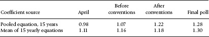
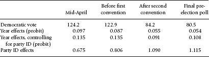
Table 7.2 shows that the impact of party identification on individual vote choice does grow over the campaign timeline. The first row contains the probit coefficients from four time-specific equations that predict respondents’ vote intentions from their party identification plus year dummy variables to control for year effects. The second row contains, for each time point, the average of the fifteen party identification coefficients predicting the vote from partisanship for the specific Gallup data set. In each case the coefficients grow over the campaign. As the campaign evolves, party identification increasingly accounts for voters’ relative attraction to the Democratic and Republican candidates compared to other factors that motivate their vote.
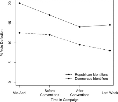
Figure 7.4 shows this pattern directly, as partisan “defections” over the campaign timeline. For both Democrats and Republicans, it depicts the percentage (among major-party voters) of party identifiers who defect by voting for the other major party. The numbers are averages for the 15 elections, weighting each election equally. In April of the election year, about 20 percent of Democrats and 15 percent of Republicans tell Gallup that they intend to defect. By the final poll, each defection rate drops by about a fourth from its level in April.
The substantive implication is that over the presidential election campaign, voters increasingly consult their partisan dispositions in deciding their candidate likes and dislikes—and ultimately their presidential vote. Candidates who find themselves as underdogs in the early polling can count on many of their disaffected partisans to eventually drift back “home.” Meanwhile, candidates enjoying a large lead will find their supporters becoming even more enthusiastic. For polling trends over the campaign, the former dynamic is of greater consequence than the latter since it can cause the greater electoral movement. That is, there are more disaffected partisans to return home on the losing side than the winning side. This dynamic may not be sufficient to upend the outcome of the impending election, but it can help to make the contest closer, as we spelled out in chapter 3.
Table 7.2 Probit coefficients predicting the vote from party identification at four campaign time points
Source: Data are from Gallup polls via iPoll.
Note: The pooled equations include year dummies. From the year-specific equations, the coefficient grew in 31 of the 45 time point-to-time point comparisons. The coefficient shrunk in 12 instances, with 2 virtual ties. Each data set contains over 1,000 voting respondents.
Figure 7.4. Vote defections by time in campaign. Times are mid-April, before conventions, after conventions, and final days of campaign. Observations are averaged from Gallup polls over fifteen elections, 1952–2008.
The previous discussion is subject to an obvious critique: if party identification becomes more closely tied to the vote over the campaign, can we be sure of the causal story? The results in table 7.2 could be symptomatic of voters increasing their excitement over their favored candidate to the point of claiming to identify with their favorite candidate’s party, as was raised earlier. It is plausible that this reverse causation is a part of the causal story, but probably not the main part. Consider that party identification is stable, like vote choice, over time. Also consider from chapter 6 that, across elections, the national division of party identification is not strongly correlated with the presidential vote.
As a useful crosscheck, however, we can look at other indicators of the “internal” fundamentals by exploring the impact of demographic factors over the campaign. Even collectively, demographic variables like race, economic status, and religion do not have the predictive power of party identification. They have, however, the advantage of being virtually constant for individual voters over the campaign, and thus immune to reverse causality. It cannot be argued that voters’ group characteristics are affected by the respondent’s vote choice. If we find that demographics increasingly predict the vote over time, the causal interpretation can only be that voters increasingly incorporate interests emanating from their group characteristics into their voting decisions as the campaign progresses.
We perform a demographic analysis in very similar fashion to Gelman and King’s (1993) presentation. Whereas Gelman and King examined a considerable density of polls from 1988, we examine four polls in each of fifteen elections. All of the sixty data sets in our repertoire contain a sufficient number of demographic variables to construct a probit equation predicting vote choice from demographics. The demographic variables included in the data sets vary across years and to some extent within years as well. To test specifically for a growth in the importance of demographics over the campaign, we include for each year those relevant demographics that are in all four of our Gallup surveys for that year. This means that for some years the demographic equations will predict better than for other years as an artifact of the number of relevant variables included in the equations. Our interest, however, is not in how much of the variance we can explain by demographics, but rather in how much the explanation grows from April to November in the specific elections.
Instead of showing the details of these sixty equations, we summarize each equation’s predictive power by use of the McKelvey and Zavoina (1975) “pseudo R-squared.” The pseudo R-squared is the estimate of the degree to which the demographic equation statistically explains the unobserved, latent, “propensity to vote Democratic.” This estimate is accomplished by first computing the variance of the predictions from the equation. Since the unexplained variance is set to 1.00, the proportion of the variance explained is the equation-induced variance divided by 1 plus the equation-induced variance.
Table 7.3 Pseudo-R2 from probit equations predicting the two-party vote from demographic variables at four campaign time points in 15 presidential elections, 1952–2008
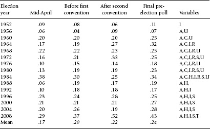
Source: Gallup Polls via iPoll.
Note: The probit equations predict the two-party vote from a series of dummy variables. All equations include dummies for southern white, not high school graduate, college graduate, woman, and African American. Other dummies are included for some but not other years: A = age (under 30, over 64); C = city; H = Hispanic; I = income (top third, bottom third); R = religion (Catholic, Jewish, other); S = single; T = church attendance; U = union household. Dummies are included for the year only if they are present in all four surveys.
Table 7.3 presents the findings. Not too much should be made of the differences across years, since the variables differ considerably from year to year, as discussed. The pattern of interest is the over-time trend within each campaign. The evidence is clear: in every election year, the explained variance increases. On average, the proportion of the explained variance from demographics increases by almost 25 percent from April to November.8 If we keep in mind that the explained variance from a probit equation is affected by the unobserved sources of variance in the latent dependent variable, the growing importance of demographics over the campaign may actually be underestimated. This is because the variation in individual assessments of relative candidate attractiveness (utility) presumably grows over the campaign, which increases the unexplained variance.
The result is that voters’ preferences are more predictable as the campaign goes on. Early in the campaign year, survey respondents indicate their candidate preference by what is in the news plus their political predispositions. As the campaign progresses, their political predispositions take on greater force. Among the specific variables, the growth in impact tends to be in variables strongly tied to partisanship. In particular, blacks, Hispanics, and Jews appear to become more Democratic over the campaign. So do women (relative to men) from about 1980, when the gender gap first came into serious play. On the other hand, the rich-versus-poor split does not expand much over the campaign.
It is instructive that in those instances in which a candidate’s demographic characteristics affected the campaign dynamic, voters who shared the candidate’s unique demographic feature respond positively from the outset of the campaign. In our Gallup poll data from 1960, Catholic John Kennedy’s support from Catholics was as strong in April as in November. In 1976, Georgia’s Jimmy Carter drew consistent support from southern whites from April to November. And already by April 2008, African Americans supported Barak Obama over John McCain to an overwhelming degree.9
We have seen that the internal fundamentals of the election—those forces that guide voters toward their personal predispositions—increasingly influence vote choices as the campaign progresses. But what about the leap from the late campaign to Election Day? Section 7.1 showed that the candidate preferences (of ANES respondents) are very stable from early in the fall campaign to Election Day. But what compelled 5 percent of the respondents to switch their candidate preference between the early fall and Election Day? In the ANES panel, 16 percent expressed a pre-election intent to vote for a major-party candidate but then failed to do so. Why did they stay home? Still another 12 percent reported lacking a preference for a major-party vote choice pre-election but then proceeded to vote Democratic or Republican on Election Day. Why did they show up on Election Day?
Section 7.2 showed that vote choices become increasingly consistent with voters’ demographics and partisanship as the campaign progresses. This we see as voters responding to the lure of their internal fundamentals. We might think that this process advances further on Election Day, as voters “come home” to their basic partisan and demographic dispositions. Our analysis of the ANES panel, however, suggests that this is not the case. Panelists who expressed a vote intention during the campaign did not continue to evolve toward their internal fundamentals on Election Day. If anything, the “dropouts,” whose preferences are recorded during the campaign but who do not vote, appear more responsive to the internal fundamentals than the “walk-ins,” who make a late decision to vote.
ANES measures party identifications during the pre-election interview. If the influence of partisanship surges between the campaign and Election Day, we would expect to see party identification correlate more with actual vote decisions than with pre-election preferences, but by any test, the answer is no. In fact, in 9 of the 15 elections, the party identification probit coefficient is greater for pre-election vote intentions than for vote choice.
An obvious interpretation is that the influence of partisanship decays somewhat from late in the campaign until Election Day. It also is possible, however, that the influence of party actually grows, but the evidence gets distorted as an artifact of its measurement during the pre-election interview. That is, the vote–partisanship correlation could be dampened because Election Day vote choice and party identification are measured at different times.
Demographics seemingly are unaffected by measurement timing, and the late-campaign growth of its influence on voters deserves a closer look. For each election, we estimated a probit equation predicting September-October pre-election vote intentions and another predicting the vote decision, from an identical large set of demographic dummy variables. In contrast with our earlier analysis of vote intentions at different points in the election year, the same variables are in all of the equations, except for a Hispanic dummy that starts in 1984 when ANES began to ask respondents about a possible Hispanic heritage. The samples for each year are limited to those panelists who expressed both a pre-election vote intention and a vote decision for a major-party candidate. The variables and their coefficients predicting the vote are shown in figure 7.5. The variables include age, region, income, race, religion, education, and gender.
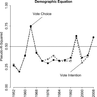
Figure 7.6 displays the pseudo R-squareds for the equations predicting the vote and also those predicting vote intentions. Clearly, the explained variance from demographics grew over the half-century of analysis. The important fact on display here, however, is the comparison of the pseudo R-squareds in each year, which demonstrate the explanatory power of demographics predicting pre-election vote intentions and Election Day vote choices. Unlike what we find for vote intentions over the campaign year using Gallup polls at different stages of the timeline, here we find no systematic growth in the explanatory power of demographics going from pre-election vote intentions to vote choice in the ANES panels. Demographic variables predict the vote no better than they predict pre-election vote intentions. The results imply that the increasing crystallization of preferences based on demographic fundamentals does not persist to the very end of the cycle. Indeed, the structuring of preferences is essentially complete by the time of the formal campaign in the fall, when ANES respondents are first interviewed.10
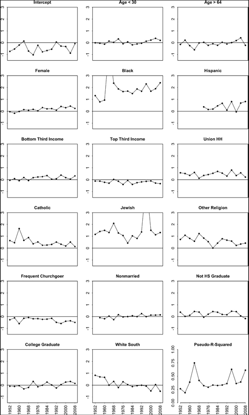
Figure 7.5. Effects of demographic variables on vote choice among ANES respondents, 1952–2008. Values are probit coefficients.
Figure 7.6. Comparison of pseudo R-squared predicting pre-election vote intentions and post-election vote choice. Equations are based on ANES respondents who offered a vote intention in the pre-election panel wave and reported a vote choice in the post-election panel wave.
Previous chapters have raised the puzzle of variance compression, whereby the variance of aggregate vote intentions—and then the vote division itself—shows a decrease over the campaign timeline. Why, we ask, does the partisan division of vote intentions tighten over the campaign timeline? And why is the Election Day verdict generally by a slimmer margin than found in even the final polls of the campaign? The analysis of individual-level data from the Gallup polls and the ANES pre- to post-election panels helps to explain. We consider first the compression of vote intentions from April to November by analyzing individual respondents in the sixty Gallup polls. Then we turn again to the fifteen ANES pre- to post-election panels to understand the compression of the vote variance on Election Day.
Like trial-heat data generally (see chap. 2), the set of 60 Gallup surveys shows a decline in the aggregate yearly variance of vote intentions. An analysis of the individual data from these surveys reveals why this is so. Table 7.2 (in the first row) showed that, across the 15 elections, the impact of party identification (relative to the unobserved error term) increased over the four points in the timeline. This finding was based on equations that included dummy variables for year effects. These year effects are relevant because they incorporate the external fundamentals of the campaign. As vote intentions became more driven by internal partisanship, the impact of external campaign-specific forces also grew during two of the three comparison periods. The demonstration follows in table 7.4.
For reference, the first row of table 7.4 shows the cross-sectional variances of aggregate vote intentions (across years) among the Gallup respondents at the four points in the timeline. There are no surprises. Just as for our global poll of polls (chap. 2), the variance of the vote for our selected Gallup samples declines, especially over the convention season. The second row of table 7.4 shows the variances of year effects from probit equations predicting the vote from year dummy variables alone. Again, we see the variance decline over time, especially from before to after the conventions. Pre-convention, the election year can account for almost 10 percent of the variance in the propensity to vote Democratic. Post-convention, this proportion is cut virtually in half.
The third row of table 7.4 shows the variances of the dummy year variables, now controlling for individual-level party identification. The variances in row 3 represent year effects relative to within-year sources of individual variation other than partisanship. We can think of this year-specific variance as the electorate’s aggregate relative utility for (liking of) the Democratic candidate versus the Republican candidate, independent of partisanship, relative to the within-year variance of individual voters’ relative utility.
Recall that probit is normed so that the unexplained variance always equals a constant, 1.0. Yet we presume that, if we could measure it, this unobserved variance of individual-level relative utility (liking) for the candidates would increase over the campaign timeline due to learning. This follows from our discussion in chapter 3. It also follows from that discussion that we would expect the aggregate variance of net campaign effects to grow at about the same rate over the campaign as the growth of individual-level unobserved variance. With the unobserved variance calibrated in constant units in probit, the expectation is that the aggregate variance (year effects) would keep pace by also staying constant over the timeline.
Table 7.4 Variances of aggregate vote intentions over the campaign timeline
Source: Data are from Gallup polls.
Note: All variances are calibrated as the percentage of the variance in the latent variable, the propensity to vote Democratic, as a proportion of the unexplained variance. Variances of year effects are normed to weigh each year equally, independent of year sample size in the Gallup meta-survey.
We see this in two of the three periods of change. Relative to the individual-level variance, the external variance from year effects stays constant April to pre-conventions and even grows slightly post-conventions to election eve. This is indirect evidence that external campaign effects on vote intentions actually increase under normal campaign circumstances even though the observed variance of the vote declines.11
The convention season provides a strong exception. During that crucial interval, even with partisanship-adjusted year dummies, the year-effect variance declines. This implies that the variance of individual-level relative utility (affect) for the candidates grows at a faster rate from the conventions than does the net change in the net utility at the national level. In effect, individual voters’ impressions of the candidates must be evolving at a faster rate than the net aggregate verdict. The information from the conventions induces considerable churning of the vote in both partisan directions, perhaps even more than the considerable amount of aggregate change would suggest.
Finally, we observe the fourth row of table 7.4. Here, we see that, with year effects controlled, party identification effects increase over the time line and in fact more than double in size. This is crucial. As we saw in the previous section, voting becomes more determined by partisanship as the campaign progresses. In fact, relative to the unobserved individual-level variation in net candidate attraction (the unobserved residual), partisan-ship’s variance more than doubles from April to November.
Let us put the parts together to offer an interpretation of the declining variance of vote intentions over the campaign timeline. Setting aside convention effects for special treatment, we observe that before and after the conventions, the aggregate cross-election variance of net relative candidate attractiveness keeps pace with the within-election variance of relative candidate attraction. Meanwhile, the effect of partisanship grows at a much faster pace than relative candidate attraction. The growth of partisan effects (observed as keeping pace with residual individual level effects) means that over the campaign, partisan voters “come home” to their party after a possible initial attraction to the opposition. Put simply, the vote margin keeps getting closer because party identification pushes the vote toward the center (e.g., a normal vote based on the division of partisanship) faster than candidate evaluations push the vote away.12
The pre- to post-election panels in the American National Election Studies offer a unique opportunity to test for the sources of the compression of the aggregate vote division between the fall campaign and the final vote. With ANES data, aggregate pre-election vote intentions and the aggregate vote division show variances of 10.05 and 6.86, respectively. The pre-election variance is similar to that reported for late surveys in chapter 2. The aggregate reported vote is similar to that for the actual vote. Thus, the panel shows the usual Election Day compression of the aggregate vote, with the variance dropping by about one-third. So let us use the leverage of panel data to decipher why the vote division (on Election Day or in post-election polls) tends to be closer than the division of vote intentions among respondents, pre-election.
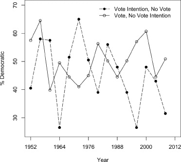
The answer is not an increase in the role of partisanship between the pre-election poll and Election Day. The discussion in section 7.3 would seem to dispel that plausible idea. (Party identification measured during the campaign predicts vote decisions no better than it predicts vote intentions.) Instead, we can explain most (but not all) of the variance compression from the contrasting behavior among ANES respondents who are dropouts, who offer vote intentions but then do not vote, versus walk-ins, who initially abstain but do vote. The contrasting behavior of these two groups—the no-shows and the unexpected participants—is shown in figure 7.7.13
The vote intentions of the seemingly likely voters who do not follow through tend to favor the short-term forces of the day. They favor the eventual winner and then do not show up on Election Day. Their inclusion in polls serves to inflate the variance of aggregate vote intentions across elections. The variance of vote intentions for dropouts is 13.69, compared to 9.88 for eventual votes. This evidence suggests that when eventual dropouts are interviewed pre-election, their responses may be influenced more by short-term forces than those of actual voters. Consider in contrast the smaller sets of respondents who (a) either do not intend to vote or have not decided on a major-party candidate but who (b) do vote for the Democrat or Republican on Election Day. These late-deciding walk-ins tend to divide close to 50–50 on Election Day, thus deflating the variance of the aggregate vote. The variance of their aggregate vote decisions is a mere 5.68, less than half that for the vote intentions of the dropouts.
Figure 7.7. Campaign vote intentions by nonvoters and votes by those without pre-election vote intentions, 1952–2008. Among ANES respondents who were successfully interviewed post-election.
We can see the net result by comparing the aggregate variance of vote intentions and the Election Day vote for only those respondents who both expressed a pre-election vote intention and voted. When measured for these committed respondents, the aggregate variance is virtually constant from pre-election to Election Day. For this set of voters, the variance of aggregate vote intentions is 9.88, whereas the variance of the aggregate Election Day vote is 8.84. Although there is still daylight between these two figures, we see that for committed voters, the variances of the pre-election vote intentions and the final vote are similar. Among this set of voters, there is little variance compression. The removal of dropouts and walk-ins reduces the variance gap between pre-election vote intentions and Election Day results by about two-thirds. The contrast between the no-shows and the unexpected voters is responsible for the bulk of the variance differential.
Even though pollsters take great pains to restrict their pre-election polls to likely voters, many slip through their screen. The good news (for pollsters) is that these erroneously counted nonvoters generally do not have preferences opposite the partisan tendency of the actual electorate. The bad news is that their support for winning candidates appears to be exaggerated. This results in some confounding of both the pollster’s analysis and our attempt here to understand the electoral verdict.
Unlike preceding chapters, this chapter has focused on individual voters in national trial-heat surveys. We have learned that presidential vote choices are quite stable between elections and during presidential campaigns, and that the stability increases as the campaign unfolds. Over the campaign, vote choices are increasingly predictable from the internal fundamentals of partisanship and group identities. It is a general pattern, found over fifteen presidential election campaigns. As voters return to their partisan roots during a presidential campaign, the aggregate division of vote intentions gravitates toward its normal level. And on Election Day, the verdict closes further, as the short-term forces of the campaign attract many survey respondents who ultimately do not vote.
The analyses in this chapter take us a long way toward explaining a puzzle that has guided our work. Why does the cross-sectional variance of vote intentions decline over time? The pattern mostly reflects the internal fundamentals: voters with different partisan dispositions return to their partisan roots. As a result, as the campaign progresses over the timeline, voters behave less like Independents and more like committed partisans. With a verdict based increasingly on partisan dispositions, the aggregate result looks more like a partisan vote as Election Day approaches. The very late decline in variance reflects another factor, however. We see that many eventual nonvoters say they intend to vote in pre-election surveys, and these dropouts tend to vote for the winner. This expands the variance of pre-election aggregate vote intentions beyond what results on Election Day. Meanwhile, another group of voters decides to vote at the last minute. These walk-ins, as late deciders, tend to vote 50–50, thus serving to compress the variance of the aggregate Election Day vote.