The previous chapter documents an important fact: with some interesting variation across election years, the electorate’s presidential vote intentions evolve over the course of a presidential campaign. We know this because poll results within an election year vary far more than would be expected by sampling error alone. But how should we model the dynamics of electoral preferences over the presidential campaign?
One possibility is that preferences start at some pre-campaign set point and then move unpredictably from that point on, driven by the unforeseeable actions of the two presidential campaigns. This would seem to be the strongest case for campaign effects. The electorate’s opening verdict is some plausible starting point in terms of the relative strengths of the two candidates and then careens uncontrollably as a function of which campaign outperforms the other and by how much. The model is hardly attractive, particularly if one envisions the relevant effects to be a series of distortions, gaffes, and hoopla that can only serve to guide the electorate away from a choice determined by the “fundamentals.” It also is not very credible, as we know that outcomes are, at least to some extent, predictable in advance. Is there another, more attractive, interpretation of how campaign effects work?
Most scholarly accounts of campaign effects are quite different from that of the previous paragraph. In these accounts, campaigns move the electorate toward an outcome driven by the fundamentals, not away. This is what Bartels (2006) calls the “priming” function of campaigns. Others refer to enlightenment or “learning.” (We have already noted how priming and learning may be related.) The story goes that early in the campaign, voters allot minimal attention to campaign news and develop only superficial impressions for the pollsters to analyze when they monitor preferences. Then, as the campaign progresses, voters start to focus on the fundamentals of the campaign, which (recall from chap. 1) come in two different flavors—“internal” ones that are specific to individual voters and “external” ones that reflect the political and economic context of the election. The campaign effectively delivers these fundamentals to the voter rather than distorts the outcome away from what they would predict. The view that campaigns cause voters to attend to the fundamentals is an established perspective in the literature. Can we accommodate it within our conceptualization of the voter preference time series?
For now, we hold off regarding the content of these fundamentals and concentrate on the dynamics of aggregate vote choice over the campaign. We consider how voters might (or might not) be influenced by forces we depict as fundamentals. For instance, is the variation of the vote division during the election campaign nothing more than episodic and transient shifts that dissipate within days only to become extinguished by Election Day? Or does it represent an accumulation of (perhaps small) voter responses to the campaign, which carry the Election Day verdict far afield from what the polls show early in the campaign? Further, do shifts in preference respond to the same or different types of stimuli at different stages of the campaign?
The discussion must venture into the realm of time-series statistics. Time-series analysts take seriously the task of diagnosing the statistical properties of their data—for example, is the series stationary or integrated? These queries are typically motivated by statistical concerns that rarely interest the lay reader—for example, given the data characteristics, what kind of statistical methodology should be performed? Here, our interest is substantive, not statistical. In describing the time series of campaign preferences, we hope to capture substantive information about preference change during the campaign.
We can only tread lightly into the arena of time-serial statistical diagnostics. The data allow no more. Polls are conducted irregularly during campaigns, rather than at regular intervals such as every day or even every week. And, as we discussed in chapter 2, polls are subject to considerable measurement error. Furthermore, we must confront the fact that national aggregations of candidate preferences represent the composite of millions of individual-level time series describing individual voters.
We start by modeling the individual voter’s decisions that comprise the national vote. Consider the voter’s choice at some arbitrary starting point early in the campaign time series. Without the constraint of actually measuring it, we can consider this choice as the relative preference for Candidate A versus Candidate B, that is, the degree of attraction to A minus the degree of attraction for B. One could consider this score as an attitude—degree of relative liking—or as the voter’s relative utility as an anticipated benefit from one candidate relative to the other. The exact conceptualization does not matter. We set the scale of hypothetical measurement so that high scores are pro–Candidate A and low scores are pro–Candidate B. The zero point is the threshold of vote choice. If the voter’s momentary score is greater than zero, she votes for A; if less than zero, she votes for B.
Now let us imagine this voter’s hypothetical time series of daily readings over the course of the campaign, starting with our earliest readings in April (or before). Early in the election year, a respondent in a trial-heat poll might not have given much thought to her relative preferences for the likely party nominees, but is able to retrieve sufficient information from memory to state a preference for one of the candidates. What would go into this choice?
For now, let us assume that the voter has a basic disposition of relative liking, built on partisan experience plus some contextual information regarding the current political times and the early information about the candidates. If the voter’s choice is monitored regularly, this fundamental disposition anchors the voter’s choice. Over time, on average, the best guess regarding our voter’s relative preference is this disposition. But our voter’s relative preference of the moment may depart from the disposition. From time to time, our voter might be swayed by new information in her political environment that compels at least a momentary departure from the basic disposition. This short-term variation might be due to personal discussions or information in the mass media or even the silent contemplation of political issues. We can think of these sources as a series of shocks or innovations to a person’s thinking. The half-life of these shocks could be fleeting, or they could be long lasting. If they become a permanent part of the person’s political memory, they not only change the short-term response but the voter’s long-run disposition as well for Candidate A over Candidate B (or vice versa).
Consider next a collection of voters, as described, with individualized dispositions and short-term variation around these dispositions. If we could measure their individual scores on the Democratic minus Republican scale, we could monitor their average over time. If individual dispositions are constant and short-term variation is idiosyncratic to the individual, then the aggregate mean value would be nothing more than a constant. (The individual variation would cancel out.) Similarly, the proportions preferring the Democratic and Republican candidates, above and below the zero threshold, would be constant. To create aggregate change, therefore, the campaign innovations must move in phase, at least partially, with voters responding somewhat in tandem to common stimuli. In other words, events must affect individuals in such a way to produce a net partisan benefit rather than be neutral.
These common shocks then produce shifts in aggregate voter preferences over the campaign. If these common shocks or innovations are temporary in nature, their influence on the Election Day outcome is minimal, as what matters in the final analysis is the division of constant voter dispositions (plus late shocks). The campaign does have an impact on the outcome, but only at the end of the timeline. If, on the other hand, the campaign-induced shocks are long lasting or even permanent, their impact persists until Election Day. In this latter case the campaign matters continually, over the entire timeline.
Thus, we can conceptualize election outcomes as essentially a function of the collective voter dispositions present at the start of the campaign plus their change (if any) over the campaign. Of course, even with polls conducted regularly over the campaign, we cannot directly measure the march of voter predispositions. Viewed through a filter of survey error, the electorate’s vote division reflects a combination of long-term voter dispositions plus short-term variation that may masquerade as meaningful change. And, of course, the polls do not measure the relative preferences themselves. They measure only the division of probable or likely voters by their presidential choice of the moment as Democratic or Republican. It is to the properties of this aggregate time series that our discussion turns next.
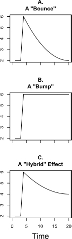
We start with the knowledge that because the electorate’s vote division does sometimes change over the course of the campaign, campaign events (broadly defined) must be exerting some sort of impact. In the language of popular commentary about campaigns, the question is: Do these shocks from campaign events take the form of temporary “bounces” or permanent “bumps”? Figure 3.1 illustrates the distinction. Bounces dissipate with time, as depicted in figure 3.1A. They matter on Election Day (if at all) only when they occur late in the campaign. Bumps persist, as illustrated in figure 3.1B. Because they last until Election Day regardless of when they occur, they are more consequential.
Figure 3.1. Bounces and bumps.
Bounces or bumps? The answer is important because it reveals the relevance of campaign shocks. As a series of short-term bounces, the campaign-induced shocks to the electorate’s collective choice over the campaign have little net impact on the final outcome. As an accumulation of bumps, however, all campaign-induced shocks affect the outcome whether they occur early or late in the campaign. With only bounces, the election verdict is largely a reversion to a preordained equilibrium value rather than transient campaign events. With only bumps, the election verdict is the sum of campaign events, with no equilibrium. Of course the truth might be that campaign shocks generate both short-term ripples (bounces) and long-term waves (bumps). Figure 3.1C illustrates this hybrid. For practical purposes, long-lasting bounces may be indistinguishable from permanent bumps.
If campaign effects are bounces, over-time preferences must revert to an “equilibrium” mean value that represents in some way the “fundamentals” of the campaign. Here the final Election Day outcome is the simple sum of this equilibrium plus the effects of late events that have not fully dissipated by Election Day. If campaign effects are bumps, conversely, they persist and affect the outcome. In effect, the election outcome is the sum of all the bumps—perhaps small in size—that occur during the campaign. The answer may be that campaign events produce both bounces and bumps. It may be that some effects dissipate and others last. It is the bumps and not the bounces that matter in the long run. With both bumps and bounces, the accumulated bumps provide a moving rather than stationary equilibrium. The bounces are but short-term noise.
This section introduces a series of mental experiments in which we imagine that we can observe the actual time series of vote intentions over the campaign. Let us assume that we have trial-heat polls at regular intervals over the course of a campaign. Let us further assume that we have perfect polls, that is, no bias, sampling error, and so forth. Furthermore, let us assume that these perfectly measured readings are at regular intervals, perhaps daily, throughout the campaign. What would they show?
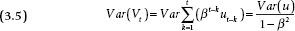
Consider the time series of the electorate’s aggregate vote division (Vt) during the election cycle to be of the following form:
where Vt is the vote percentage for Candidate A rather than Candidate B and ut is a series of random campaign shocks.1 That is, preferences on one day are modeled as a function of preferences on the preceding day and the new effect of campaign events, broadly defined. The specific events from one day could trigger a series of delayed shocks to voter preferences in subsequent days, as the media message reverberates. By the same token, the shock emitted on any given day could include the delayed reaction to events from earlier days. Equation 3.1 allows us to characterize different general models of campaign dynamics.
Equation 3.1 models a conventional AR1 autoregressive process. The definition of an AR, or autoregressive, process is that the variable of interest (e.g., the vote division) is a function of its value at the previous time period plus a new random shock for the new period. What makes it an AR1 model is that apart from its lagged value at t − 1, that is, the previous period, the variable’s history does not matter. That is, if we know (without error) the preferences at the previous reading (t − 1), preferences at earlier dates (t − 2, t − 3, etc.) add no further useful information. Similarly, if we know (without error) the preferences further back in time at t − m, preferences at earlier dates (e.g., t − m − 1, t − m − 2, etc.) do not matter. (A convenient conceptualization, the AR1 assumption is relaxed below when we consider the vote as a composite of two separate time series.)
The variance of ut reveals the typical magnitude of the daily shocks to voter preferences. As long as the ut variance is nonzero, we know that campaigns affect voters, and the larger the variance the greater the immediate effects. The expectation that campaign effects are present in US presidential elections is standard, as discussed in chapter 1.
The existence of campaign shocks provides only half the story, however. We also want to know about dynamics. That is, are shocks permanent or do they decay with the progress of time? In theory, these dynamics are directly evident from the coefficient β in equation 3.1. If β is between 0 and 1, the process is what is called a “stationary series” in time-series parlance. Two features of a stationary series are a constant variance over time and a reversionary equilibrium value. If β equals 1.0, the process is not stationary but rather an integrated series, otherwise known as a “random walk.” Two features of a random walk are a growing variance over time and the absence of a reversionary equilibrium. Whereas with a stationary series, expected change is in the direction of the long-term mean—the more off equilibrium, the greater the reequilibration—with a random walk the expected change is zero. That is, scores are as likely to go up as down.2
The distinction between stationary and integrated series matters for our understanding of campaigns. A stationary series is an accumulation of ever-receding bounces. An integrated series is an accumulation of bumps. If electoral preferences over a campaign form a stationary series, current preferences are largely a function of the reversionary equilibrium (long-term dispositions) value plus recent bounces. How disproportionately recent shocks matter compared to those from the more distant past is a function of the size of β. The closer β is to 0, the more only recent events matter. The closer β is to 1.0, bounces from the remote past continue to live. In extreme, when β = 1.0, the bounces become bumps and accumulate to form an integrated series, otherwise known as a random walk. If electoral preferences comprise an integrated series, current preferences are equally a function of campaign shocks past and present.
Consider first the possibility of a stationary series. With 0 ≤ β < 1, effects decay over time. As an “autoregressive” (AR) process, preferences tend toward the equilibrium of the series, which is α / (1 − β). If the division is greater than its equilibrium value, it will decline over time; if it is below the equilibrium value, it will increase. The equilibrium does not represent the final outcome, however. What happens on Election Day also will reflect late campaign effects that have not fully dissipated by the time voters go to the polls. The degree to which late campaign effects do matter is evident from β, which captures the rate of carryover from one point in time to the next. The smaller the β, the more quickly campaign effects decay and the less they matter on Election Day.
With aggregate preferences over a campaign behaving as a stationary series, predicting Vt from Vt−1 one period earlier can be described by the following equation:
where V* is the equilibrium or long-term mean. (Recall that V* is α /(1 − β), where α is the intercept in equation 3.1. With a further algebraic transformation, equation 3.3 sets the dependent variable to be the t − 1 to t change in electoral preferences.
where Δ Vt = Vt − Vt − 1. Note that preference change consists not only of the new shock ut but also the lagged departure from equilibrium (Vt−1 − V*) times the requilibrating rate (β − 1), which will be less than 0. To be absolutely clear, when Democratic vote intentions at time t − 1 are above (below) the equilibrium value, we predict a drop (rise) in Democratic vote intentions at time t. The smaller the β, the greater the requilibrating rate (β − 1), and so the larger the drop.
In the extreme, when β approaches 1.0 there is no reequilibration, leaving preference change as simply the new shock. The long-term electoral change then is the summation of accumulated shocks without reversion, or an integrated series in which all past shocks matter equally with no forgetting. With β = 1, equations 3.2 and 3.3 simplify to
and
Because shocks decay in a stationary series, the variance is a function of both the variance of the ut shocks and also the autoregressive parameter β. Asymptotically (in the long run), the variance of a stationary series is constant, that is, “stationary”:
As β reaches 1, however, the long-run variance of Vt increases. Whereas the variance of a stationary series is constant, the variance of an integrated series continues to grow.
Should vote intentions in presidential campaigns be modeled as a stationary series or as a random walk? As we will see, the off-the-shelf application of either model is unsatisfactory, and further tinkering is required. Consider first the potential of modeling voter preferences over a series of presidential campaigns as a set of stationary series.
In general, if aggregate preferences follow a stationary series, predicting Vt from Vt−m at m days earlier can be described by the following equation:
To the extent that β is less than 1.0, and the t − m time gap is large, the forecast for time t at time t − m reverts to V*, the constant term representing the fundamentals.3 In a certain sense, then, the campaign does not matter until close to Election Day in this model. Meanwhile, since the Election Day outcome would become the natural baseline from which earlier forecasts are measured, there would be a natural tendency to mistake the outcomes as the fundamentals rather than a combination of fundamentals and late campaign effects.
As we have seen, to depict the campaign vote division as a stationary series is to depict campaign effects as a series of campaign bounces. The problem is that a stationary series maintains the equilibrium as a constant as if campaigns are governed by an underlying equilibrium value that is evident at the start of the series and never changes. It is not very plausible that the electorate’s collective long-term dispositions are set in concrete by forces that are in place by the start of the campaign.
Now, consider the possibility that, rather than as a stationary process, the electorate’s vote division moves throughout the campaign as a random walk. With β = 1, campaign effects actually cumulate. Each shock makes a permanent contribution to voter preferences. There is no forgetting. As a “random walk”—what also is referred to as an “integrated” process—preferences cumulate over the election cycle and become more and more telling about the final result. The actual outcome is simply the sum of all shocks that have occurred during the campaign up to and including Election Day.4 An attractive aspect of conceptualizing campaign dynamics as a random walk is that it allows campaign effects to persist throughout the campaign, lending the final outcome a certain degree of unpredictability given the initial values.
There is, however, one feature of a random walk that appears to violate the nature of the actual data. With a random walk, the cross-sectional (between-elections) variance of the vote division must increase with time. The farther along in the campaign cycle, the farther apart are the divisions in different campaigns. Observed over many campaigns, we would see a tendency for races to become increasingly one-sided rather than tighten as the campaign progresses. This expansion of the cross-sectional variance is not consistent with the facts. In reality, as we saw in chapter 2, the cross-sectional variance has a tendency to compress over time. At first blush, therefore, it seems that aggregate electoral preferences could not evolve as a random walk.
We must consider the possibility that vote preferences combine long-term bumps and short-term bounces. In other words, we can conceptualize the series as the addition of a random walk as the moving equilibrium ( ) plus a short-term stationary series (
 ) around this equilibrium:
where
and
The two parts can be combined in the following “error correction” model:
where 0 < β < 1 and et is introduced as the disturbance to  . In this model, some effects (ut) persist—and form part of the moving equilibrium —and the rest (et) decay. That is, the fundamentals move as a random walk, whereas short-term campaign forces create a stationary series of deviations from the moving fundamentals.5 Some campaign effects persist and the rest decay.
If the time series of aggregated preferences is a combination of the two processes, the integrated component takes on greater importance than the short-term variation of the stationary series. Indeed, statistical theory (Granger 1980) tells us that any series that contains an integrated component is itself integrated in the long run. The intuition is that, because of its expanding variance over time, the integrated component will dominate when viewed over a long-term perspective.6
A combined integrated series plus stationary time series makes intuitive sense. By this process, the fundamentals (V*) move toward their final evolution on Election Day. Meanwhile the vote division is also subject to short-term perturbations that may seem important at the time but do not last until Election Day. In fact our working assumption is a variation of this model. But for that to work, one important obstacle must be overcome. Since the hybrid model is dominated by the integrated series, as discussed earlier, its cross-sectional variance must expand with time, yet we observe that the actual variance contracts over time. Thus, as with a strict random walk, the hybrid model is seemingly incompatible with the fact that the variance of aggregate vote intentions declines over the timeline.
These different models of campaign dynamics are not mere statistical musings. They formalize general arguments in the literature about the role of political campaigns. What we ultimately want to know, after all, is whether the campaign has real effects on electoral preferences and whether these effects matter on Election Day. We know that preferences do change over the campaign as new shocks (along with sampling error) create changes in the polls. But do these changes persist to Election Day?
We must ask, are there permanent campaign effects that last until Election Day, and, if so, are they of a magnitude to make a difference? If there are short-term effects, we must also ask, how large are they? And, do they persist long enough to matter on Election Day? In the extreme, all influences (apart from sampling error) on the polls from early in the campaign to the end are equally eventful, signifying a very consequential campaign. At the other extreme, all campaign-season influences are transient, whereby only the most recent campaign effects are lasting on Election Day.
Statistically oriented social scientists are often conditioned to view stationary series as the natural state of affairs, due in part to their familiarity and their convenient properties. But if we model the time series of electoral choice as a stationary series, awkward questions follow. With the campaign-induced time series of electoral preferences as a set of stationary series, variation in election outcomes would be due almost solely to cross-election variation in a set of equilibrium outcomes. Since these equilibria would be stable from the arbitrary starting point of the series onward to Election Day, election outcomes would be knowable from the early polls. This would beg the question of how different equilibria could emerge before each election season as a function of early political forces only to then remain stable throughout the actual campaign. As we have seen, modeling the vote division as driven by a random walk process (with perhaps short-term variation around it) presents its questions as well, since races actually tend to tighten, not get more one-sided as the campaign unfolds.
As we set up our questions about the nature of how campaign preferences evolve over the campaign timeline, we do not demand or expect a knife-edge diagnosis whereby campaigns matter a lot or matter not at all—or that all innovations in preferences are strictly permanent or ephemeral. We expect the presence of both a long-term sequence of small bumps and a short-term set of large but then receding bounces. Moreover, the bounces might persist with a considerable half-life. When stationary effects are so persistent (β approaching 1.0), and the series appears possibly integrated, the distinction between permanent and merely long lasting is of little practical consequence (see note 3). The surprise would be if campaigns produce nothing more than short-term effects that dissipate within days.
So far our speculation about the nature of campaign preferences has ignored the role of temporal variation in the model, as if the dynamics of our various series have identical statistical properties both early and late in the election year. We could find differences over the campaign in the nature of the time series. For instance, we might find the variance of shocks increases (or decreases) as Election Day approaches. Further modification is needed, therefore, as the actual data clearly do not fit a strict stationary series, an integrated series, or their simple composite. Thus, some modifications are in order.
In this section, we consider two modifications. First, we consider the temporal implications of treating the underlying random walk in terms of aggregated voter utilities (or relative liking) rather than in the vote division itself. Second, we consider the possibility that the voters’ considerations can change over the campaign, as if the function of the long campaign is to prime the voters to concentrate on certain fundamental information at the expense of other, less relevant considerations.
As we have seen, a series that moves as a random walk (with or without short-term variation around it) would normally expand the cross-sectional variance of the vote division, as vote intentions from different years would increasingly diverge from one another as the campaign timeline progresses. How then can we modify our model to accommodate the fact that the cross-sectional variance of the vote division contracts rather than expands with time? One solution emerges from our understanding of how aggregate vote intentions evolve from individual voter assessments. The changing vote division represents the changing proportion that favors one candidate over the other, while cumulative campaign effects represent the aggregate change in voters’ relative utilities. As voters accumulate their relative utility for the two candidates (perhaps as a random walk), the flow of campaign information intensifies voters’ relative preference for one candidate over the other. As a result, the aggregate variance of individual preferences can expand at a faster rate than the variance of the aggregate mean preference. The consequence is a natural tightening of electoral contests. We call this the “intensification effect.”7
Consider again that aggregate preferences are the sum of individual vote choices. And these individual choices are the function of voters’ relative attraction to the two candidates. As a campaign evolves, with individuals’ relative liking for one candidate over another themselves a series of random walks, the variance of these individual preferences will increase. The result of this campaign intensification is fewer voters being on the fence. As the campaign progresses, campaign events create fewer vote conversions because there are fewer voters on the fence available for conversion. More conversions that do occur will flow from the candidate who is ahead to one behind, than from the one behind to the one ahead. The result is a tightening of the vote division, counteracting the expansive properties of a random walk.
To see this, suppose we could observe individual voters’ mean scores on a scale of relative liking for the parties—the degree of liking Party A minus the degree of liking of Party B—and that these relative preferences form a random walk. These random walks are largely idiosyncratic, but when they move in tandem to a common set of national-level stimuli, the mean shifts represent campaign effects. Aggregations of individual random walks must also behave as a random walk. We do not, however, observe these aggregations but rather the manifestation as a Democratic (Republican) percentage of the two-party vote (or some other variant of aggregating vote choice). Measured as an aggregation of dichotomous Democratic versus Republican choices, the prospective vote will not necessarily display the characteristics of a random walk when the variance of the underlying latent attitude is expanding.
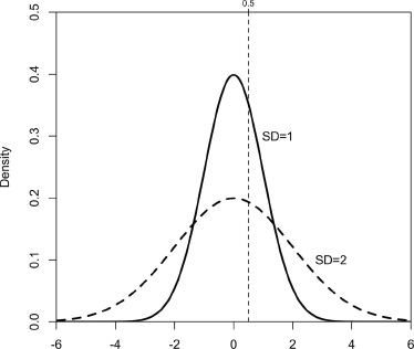
Let us conduct the following mental experiment. Assume individual latent attitudes change in the manner of a random walk, but with no net effect (neither party gains). For convenience, suppose the latent attitudes are normally distributed with a standard deviation of 1.0. Figure 3.2 illustrates this change. Assume a vote threshold of 0.5 standard deviation units, as shown in the tighter of the two normal distributions. Voters scoring higher prefer candidate B; those with a lower score prefer candidate A. This breakdown yields 69 percent for A and 31 percent for B. Now suppose that the campaign generates a further spread in latent attitudes to double the original standard deviation (increasing the variance by a factor of 4), as illustrated by the broader of the two normal distributions. If the mean attitude does not change, the threshold of 0.50 standard deviations on the original scale now shifts to 0.25 standard deviations on the expanded scale. With only 60 percent of a distribution being to the left of 0.50 standard deviations, the percentage voting for Candidate A drops from 69 percent to 60 percent, even though there is no net change in mean attitude.
Figure 3.2. The changing distribution of the two-party vote as the standard deviation of voter relative utilities doubles.
Further, consider the result if the campaign generates a small perturbation in the threshold. The proportion of the voters who shift sides will be greatest with the tighter distribution. The broader the distribution of relative utilities for the candidates at the time, the less will be the observed effect of any campaign shock when measured in terms of vote proportions.
From this exercise one readily sees that growth in the variance of voter preferences over a campaign can depress the percentage for the candidate who is ahead. And each increment of aggregate attitude change yields a diminishing impact on the percentage for each candidate. Undoubtedly such a process contributes to a slowing of any growth in the cross-sectional variance of the vote, which we measure as the dichotomous vote division. Short-term effects might be particularly affected, so that bounces decline in amplitude over the campaign.
It is certainly plausible that the individual-level variance in relative utility expands over a campaign as preferences intensify. In reality, however, do individuals’ relative preferences expand over a campaign as much as required to fully account for the declining cross-sectional variance? For a more complete accounting, we need to consider a related possibility, namely, “partisan mobilization.”
In chapter 1 we described the “fundamentals” of the election as a combination of campaign-induced “external” factors and voters’ “internal” attractors, such as their unique partisan dispositions.8 As voters strengthen their partisan leanings, further campaign events hold less sway over their vote choice. In terms of their dichotomous vote choice, strong partisans tend to be locked into their choices, whereas “independent” voters with no partisan leanings fluctuate in response to campaign news. Here is the important part. If, as many suggest, one function of campaigns is to reinforce voters’ partisan predispositions, the preferences of even mildly partisan voters become stronger over the campaign. This partial strengthening has the effect of diminishing the cumulative effect of the campaign on aggregate vote choice.
Think of a typical voter starting out the campaign as a partisan, but not very mindful of its possible implications on vote choice. This voter’s relative candidate preference will respond to the campaign news. As this information about the candidate choice accumulates, the cumulative effect on our voter’s utility calculation (or candidate affect, if you prefer) will grow. So will the chance that our weakly partisan voter will vote for the candidate of the other party. In one sense, the voter is flirting with the other party.
The complication arises as the campaign also activates our voter’s partisan identity, which pushes her candidate preferences increasingly toward her party’s candidate. As this happens, the cumulative effect of campaign information, while still present in our voter’s mind, becomes increasingly irrelevant to the vote decision. The voter becomes more committed to a candidate both because of increased campaign information and partisan activation. A crude approximation of this dual process for the individual voter is as follows:
Uit = U(Et) + φ, U(It)
where Uit = the ith voter’s relative utility for Candidate A minus Candidate B at time t,
U(Et) = the utility derived from the external fundamentals of the campaign at time t,
φ, U(It) = the utility derived from the internal fundamentals from voter predispositions, and
φt = the salience of internal fundamentals (e.g., partisanship) at time t.
As the campaign progresses, the salience parameter (φt) increases.
Assuming this is the correct model at the individual level, the macrolevel effect is for the growing partisan activation to push the vote margin toward the center. Partisan activation compresses the cross-sectional variance of aggregate vote intentions, even as the growth of campaign effects expands it. A useful way of thinking about this is to consider a set of partisan voters and a set of independent voters over a campaign. The time series of our partisan voters (equally divided between Republicans and Democrats) will show little response to campaign events. It is not that they are unaware; it is just that the news rarely pushes their choice across the threshold of the partisan divide. Meanwhile the collective choices of the independents respond freely to the campaign news. Now, consider that over the campaign the electorate as a whole becomes less like the independents and more like the strong partisans. The net effect is that the contribution of campaign effects on the time series will decline. It will not, however, evaporate. The candidate favored by the campaign will win a greater vote share than if the outcome were a strictly party-line vote. The size of the advantage, however, will lessen over time.
In the vocabulary of the American Voter authors (esp. Campbell et al. 1966), the partisan fundamentals are the “normal vote.” The cumulative campaign effects are the “short-term partisan forces,” with “short-term” applying to the specific election year. The translation of our argument is that while the short-term forces grow over a campaign, the increasing “attraction” of the normal vote diminishes their cumulative effect on the aggregate vote choice. The advantages of this partisan model are that it fits our understanding of partisanship and solves the puzzle of why the cross-sectional variance of the vote division shrinks over the campaign timeline.9
According to our model of voter decision-making, voters learn two types of fundamentals during presidential campaigns. First, the electorate’s net relative favorability of the two candidates is formed by the cumulative political news over the course of the campaign. Second, voters increasingly tilt in the direction of their partisan leanings.
In the aggregate we expect the following. Campaign effects accumulate over the long term (bumps), with declining additional shocks over the campaign. They are possibly accompanied by short-term changes due to campaign shocks of temporary impact (bounces). Overlaid on these processes, the growing intensity of voter preferences causes the vote to gravitate toward the electoral division based on partisan predispositions. The cumulative campaign shocks are still present at the end, but in diluted form.
This theorizing accounts plausibly for the declining cross-election variance in aggregate vote intentions over the campaign timeline. The net variance can compress from the growing pull of partisanship even as campaign shocks cause the variance to widen. Later, especially in chapter 7, we will see evidence that this is the correct model.
This chapter has addressed the dynamics of voter preferences over the course of a campaign. We imagine that we could perfectly observe the daily readings of the vote division and consider what the dynamics of this time series would look like. This exercise is designed to inform our examination of the actual evidence from polls, which follows.
We began by considering the vote division in terms of two standard time-series models from the statistical tool kit: a stationary series or a random walk. With a stationary series—campaign shocks as bounces—the vote division shifts around a steady equilibrium, which is in place throughout the campaign. That the campaign’s basic equilibrium remains in place throughout the campaign with this model is a source of unease. With the vote division as a random walk—campaign shocks as bumps—there is no equilibrium, so the vote can be propelled in directions unpredictable in advance. That vote margins widen instead of tighten with this model is a source of unease. Allowing a random walk combined with a lesser stationary series admits both bounces and bumps but does not solve the problem of counterfactually projecting a growing cross-sectional variance.
It is possible to model countervailing forces that work to compress the cross-sectional variance over time. Taking into account that individual voters’ attitudes intensify over a campaign helps further to slow the expansion of cross-sectional variance. The hardening of vote choices based on reinforced party identifications pushes the vote even more toward the fundamental partisanship of the electorate. The final verdict represents this partisanship plus, to a diminishing extent, the cumulative fundamentals of the campaign content.
One seeming oddity is that the cross-sectional variance of the vote is at its height at the earliest point of the campaign timeline for which we have poll data to measure it. Voters may not know much about the forthcoming presidential contest early in the election year. Presented with the two eventual candidates as choices in an early poll, however, voters can create diverse vote divisions in different elections based on minimal information at hand. Moreover, as we will see, the early information to some extent survives and forms part of the voters’ net decision-making on Election Day.
The models presented in this chapter will be useful as we explore the actual time series of fifteen vote divisions during 1952–2008. Although at times we find the data to be frustratingly limited, they still allow us to go quite a long way. We turn next, in chapter 4, to our empirical analysis of the polls and what they tell us about the dynamics of vote divisions during presidential election campaigns.