Risk and expected return are the key players in the game of active management. We will introduce these players in this chapter and the next, which begin the “Foundations” section of the book.
This chapter contains our initial attempts to come to grips with expected returns. We will start with an exposition of the capital asset pricing model, or CAPM, as it is commonly called.
The chapter is an exposition of the CAPM, not a defense. We could hardly start a book on active management with a defense of a theory that makes active management look like a dubious enterprise. There is a double purpose for this exploration of CAPM. First, we should establish the humility principle from the start. It will not be easy to be a successful active manager. Second, it turns out that much of the analysis originally developed in support of the CAPMcan be turned to the task of quantitative active management. Our use of the CAPM throughout this book will be independent of any current debate over the CAPM’s validity. For discussions of these points, see Black (1993) and Grinold (1993).
One of the valuable by-products of the CAPM is a procedure for determining consensus expected returns. These consensus expected returns are valuable because they give us a standard of comparison. We know that our active management decisions will be driven by the difference between our expected returns and the consensus.
The major points of this chapter are:
■ The return of any stock can be separated into a systematic (market) component and a residual component. No theory is required to do this.
■ The CAPM says that the residual component of return has an expected value of zero.
■ The CAPM is easy to understand and relatively easy to implement.
■ There is a powerful logic of market efficiency behind the CAPM.
■ The CAPM thrusts the burden of proof onto the active manager. It suggests that passive management is a lower-risk alternative to active management.
■ The CAPM provides a valuable source of consensus expectations. The active manager can succeed to the extent that his or her forecasts are superior to the CAPM consensus forecasts.
■ The CAPM is about expected returns, not risk.
The remainder of this chapter outlines the arguments that lead to the conclusions listed above. The chapter contains a technical appendix deriving the CAPM and introducing some formal notions used in technical appendixes of later chapters.
The goal of this book is to help the investor produce forecasts of expected return that differ from the consensus. This chapter identifies the CAPM as a source of consensus expected returns.
The CAPM is not the only possible forecast of expected returns, but it is arguably the best. As a later section of this chapter demonstrates, the CAPM has withstood many rigorous and practical tests since its proposal. One alternative is to use historical average returns, i.e., the average return to the stock over some previous period. This is not a good idea, for two main reasons. First, the historical returns contain a large amount of sample error.1 Second, the universe of stocks changes over time: New stocks become available, and old stocks expire or merge. The stocks themselves change over time: Earnings change, capital structure may change, and the volatility of the stock may change. Historical averages are a poor alternative to consensus forecasts.2
A second alternative for providing expected returns is the arbitrage pricing theory (APT). We will consider the APT in Chap. 7. We find that it is an interesting tool for the active manager, but not as a source of consensus expected returns.
The CAPM has a particularly important role to play when selecting portfolios according to mean/variance preferences. If we use CAPM forecasts of expected returns and build optimal mean/variance portfolios, those portfolios will consist simply of positions in the market and the risk-free asset (with proportions depending on risk tolerance). In other words, optimal mean/variance portfolios will differ from the market portfolio and cash if and only if the forecast excess returns differ from the CAPM consensus excess returns.
This is in fact what we mean by “consensus.” The market portfolio is the consensus portfolio, and the CAPM leads to the expected returns which make the market mean/variance optimal.
The CAPM relies on two constructs, first the idea of a market portfolio M, and second the notion of beta, β, which links any stock or portfolio to the market. In theory, the market portfolio includes all assets: U.K. stocks, Japanese bonds, Malaysian plantations, etc. In practice, the market portfolio is generally taken as some broad value-weighted index of traded domestic equities, such as the NYSE Composite in the United States, the FTA in the United Kingdom, or the TOPIX in Japan.
Let’s consider any portfolio P with excess returns rP and the market portfolio M with excess returns rM. Recall that excess returns are total returns less the total return on a risk-free asset over the same time period. We define3 the beta of portfolio P as
Beta is proportional to the covariance between the portfolio’s return and the market’s return. It is a forecast of the future. Notice that the market portfolio has a beta of 1 and risk-free assets have a beta of 0.
Although beta is a forward-looking concept, the notion of beta—and indeed the name—comes from the simple linear regression of portfolio excess returns rP(t) in periods t = 1,2,..., T on market excess returns rM(t) in those same periods. The regression is
We call the estimates of βP and αP obtained from the regression the realized or historical beta and alpha in order to distinguish them from their forward-looking counterparts. The estimate shows how the portfolios have interacted in the past. Historical beta is a reasonable forecast of the betas that will be realized in the future, although it is possible to do better.4
As an example, Table 2.1 shows 60-month historical betas and forward-looking betas predicted by BARRA, relative to the S&P 500, for the constituents of the Major Market Index5 through December 1992:
Beta is a way of separating risk and return into two parts. If we know a portfolio’s beta, we can break the excess return on that portfolio into a market component and a residual component:
TABLE 2.1
Betas for Major Market Index Constituents

In addition, the residual return θP will be uncorrelated with the market return rM, and so the variance of portfolio P is
where  is the residual variance of portfolio P, i.e., the variance of θP.
Beta allows us to separate the excess returns of any portfolio into two uncorrelated components, a market return and a residual return.
So far, no CAPM. Absolutely no theory or assumptions are needed to get to this point. We can always separate a portfolio’s return into a component that is perfectly correlated with the market and a component that is uncorrelated with the market. It isn t even necessary to have the market portfolio M play any special role. The CAPM focuses on the market and says something special about the returns that are residual to the market.
The CAPM states that the expected residual return on all stocks and any portfolio is equal to zero, i.e., that E{θP} = 0. This means that the expected excess return on the portfolio, E{rP} = (μP, is determined entirely by the expected excess return on the market, E{rM} = (μM, and the portfolio’s beta, βP. The relationship is simple:
Under the CAPM, the expected residual return on any stock or portfolio is zero. Expected excess returns are proportional to the stock’s (or portfolio’s) beta.
Implicit here is the CAPM assumption that all investors have the same expectations, and differ only in their tolerance for risk.
Notice that the CAPM result must hold for the market portfolio. If we sum (on a value-weighted basis) the returns of all the stocks, we get the market return, and so the value-weighted sum of the residual returns has to be exactly zero. However, the CAPM goes much further and says that the expected residual return of each stock is zero.
The logic behind the CAPM’s assertion is fairly simple. The idea is that investors are compensated for taking necessary risks, but not for taking unnecessary risks. The risk in the market portfolio is necessary: Market risk is inescapable. The market is the “hot potato” of risk that must be borne by investors in aggregate. Residual risk, on the other hand, is self-imposed. All investors can avoid residual risk.
We can see the role of residual risk by considering the story of three investors, A, B, and C. Investor A bears residual risk because he is overweighting some stocks and underweighting others, relative to the market. Investor A can think of the other participants in the market as being an investor B with an equal amount invested who has residual positions exactly opposite to A’s and a very large investor C who holds the market portfolio. Investor B is “the other side” for investor A. If the expected residual returns for A are positive, then the expected residual returns for B must be negative! Any theory that assigns positive expected returns to one investor’s residual returns smacks of a “greater fool” theory; i.e., there is a group of individuals who hold portfolios with negative expected residual returns.
An immediate consequence of this line of reasoning is that investors who don t think they have superior information should hold the market portfolio. If you are a “greater fool” and you know it, then you can protect yourself by not playing! This type of reasoning, and lower costs, has led to the growth in passive investment.
Under the CAPM, an individual whose portfolio differs from the market is playing a zero-sum game. The player has additional risk and no additional expected return. This logic leads to passive investing; i.e., buy and hold the market portfolio.
Since this book is about active management, we will not follow this line of reasoning. The logic conflicts with a basic human trait: Very few people want to admit that they are the “greater fools.”6
The CAPM isn’t the same as efficient markets theory, although the two are consistent. Efficient markets theory comes in three strengths: weak, semistrong, and strong. The weak form states that investors cannot outperform the market using only historical price and volume data. The semistrong form states that investors cannot outperform the market using only publicly available information: historical prices plus fundamental data, analysts published recommendations, etc. The strong form of the efficient markets hypothesis states that investors can never outperform the market: Market prices contain all relevant information.
The CAPM makes similar statements, although perhaps from a slightly different perspective. For any investor whose portfolio doesn’t match the market, there must (effectively) be another investor with exactly the opposite deviations from the market. So, as long as there are no “greater fools,” we shouldn’t expect either of those investors to outperform the market. Efficient markets theory argues that there are no “greater fools” because market prices reflect all useful information.
We have just described the CAPM’s assumption that expected residual returns are zero, and its implication that passive investing is optimal. As the technical appendix will treat in detail, in the context of mean/variance analysis, we can more generally exactly connect expected returns and portfolios. If we input expected returns from the CAPM into an optimizer—which optimally trades off portfolio expected return against portfolio variance—the result is the market portfolio.7 Going in the other direction, if we start with the market portfolio and assume that it is optimal, we can back out the expected returns consistent with that: exactly the CAPM expected returns. In fact, given any portfolio defined as optimal, the expected returns to all other portfolios will be proportional to their betas with respect to that optimal portfolio.
For this reason, we call the CAPM expected returns the consensus expected returns. They are exactly the returns we back out by assuming that the market—the consensus portfolio—is optimal.
Throughout this book, we will find the one-to-one relationship between expected returns and portfolios quite useful. An active manager, by definition, does not hold the market or consensus portfolio. Hence, this manager’s expected returns will not match the consensus expected returns.
The CAPM is about expectations. If we plot the CAPM-derived expected return on any collection of stocks or portfolios against the betas of those stocks and portfolios, we find that they lie on a straight line with an intercept equal to the risk-free rate of interest iF and a slope equal to the expected excess return on the market μM. That line, illustrated in Fig. 2.1, is called the security market line.
The picture is drawn for a risk-free interest rate of 5 percent and an expected excess return on the market of 7 percent. The four points on the line include the market portfolio M and three portfolios P1, P2, and P3 with betas of 0.8, 1.15, and 1.3, respectively.

Figure 2.1 The security market line.
If we look at the ex post or after the fact returns (these are called realizations), we see a scatter diagram of actual excess return against portfolio beta. Figure 2.2 shows a rather small scatter of three portfolios along with the market portfolio and the risk-free asset. We can always draw a line connecting the risk-free return and the realized market return. This ex post line might be dubbed an “insecurity” market line. The ex post line gives the component of return that the CAPM would have forecast if we had known how the market portfolio was going to perform. In particular, the line will slope downward in periods in which the market return is less than the risk-free return.

Figure 2.2 An ex-post market line.
Notice that we have put P1′, P2′, and P3′ along the line. The actual returns for the portfolios were P1, P2, and P3. The differences P1 – P1′, P2 – P2′, and P3 – P3′ are the residual returns on the three portfolios. The value-weighted deviations of all stocks from the line will be zero. Portfolio P3 did better than its CAPM expectation, so its manager added value in this particular period. Portfolios P1 and P2, on the other hand, lie below the ex post market line. They did worse than their CAPM expectation.
As an example of CAPM analysis, consider the behavior of one constituent of the Major Market Index, American Express, versus the S&P 500 over the 60-month period from January 1988 through December 1992. Figure 2.3 plots monthly American Express excess returns against the monthly excess returns to the S&P 500.
Figure 2.3 Realized excess returns.
Using regression analysis [Eq. (2.2)], we can determine the portfolio historical beta to be 1.21 with a standard error of 0.24. The CAPM predicts a residual return of zero. In fact, over this historical period, the realized residual return was -78 basis points per month with a standard error of 96 basis points: not significant at the 95 percent confidence level. The standard deviation of the monthly residual return was 7.05 percent. For this example, the regression coefficient R2 was 0.31.
The ability to decompose return and risk into market and residual components depends on our ability to forecast betas. The CAPM goes one step further and says that the expected residual return on every stock (and therefore every portfolio) is zero. That last step is controversial. A great deal of theory and statistical sophistication have been thrown at this question of whether the predictions of the CAPM are indeed observed.8 An extensive examination would carry us far from our topic of active management. “Chapter Notes” contains references on CAPM tests.
Basically, the CAPM looks good compared to naïve hypotheses, e.g., the expected returns on all stocks are the same. It does well, although less well, against abstract statistical tests of the hypothesis in Eq. (2.5), where the alternatives are “reject hypothesis” and “cannot reject hypothesis.” The survival of the CAPM for more than twenty-five years indicates that it is a robust and rugged concept that is very difficult to topple.
The true question for the active manager is: How can I use the concepts behind the CAPM to my advantage? As we show in the next section, a true believer in the CAPM would have to be schizophrenic (or very cynical) to be an active manager.
The active manager’s goal is to beat the market. The CAPM states that every asset’s expected return is just proportional to its beta, with expected residual returns equal to zero. Thus, the CAPM appears to be gloomy news for the active manager. A CAPM disciple would give successful active management only a 50-50 chance. A CAPM disciple would not be an active manager or, more significantly, would not hire an active manager.
The CAPM can help the active manager. The CAPM is a theory, and like any theory in the social sciences, it is based on assumptions that are not quite accurate. In particular, market players have differential information and thus different expectations. Superior information offers managers superior opportunities. We need not despair. There is an opportunity to succeed, and the CAPM provides some help.
The CAPM in particular and the theory of efficient markets in general help active managers by focusing their attention on how they expect to add value. The burden of proof has shifted to the active manager. A manager must be able to defend why her or his insights should produce superior returns in a somewhat efficient market. While bearing the burden of proof may not be pleasant, it does force the manager to dig deeper and think more clearly in developing and marketing active strategy ideas. The active manager is thus on the defensive, and should be less likely to confuse luck with skill and more likely to eliminate some nonproductive ideas, since they cannot pass scrutiny in a market with a modicum of efficiency.
The CAPM has shifted the burden of proof to the active manager.
The CAPM also helps active managers by distinguishing between the market and the residual component of return. Recall that this decomposition of return does not require any theory. It requires only good forecasts of beta. This can assist the manager’s effort to control market risk; many active managers feel that they cannot accurately time the market and would prefer to maintain a portfolio beta close to 1. The decomposition of risk allows these managers to avoid taking active market positions.
The separation of return into market and residual components can help the active manager’s research. There is no need to forecast the expected excess market return μM if you control beta. The manager can focus research on forecasting residual returns. The consensus expectations for the residual returns are zero; that’s a convenient starting point. The CAPM provides consensus expected returns against which the manager can contrast his or her ideas.
The ideas behind the CAPM help the active manager to avoid the risk of market timing and to focus research on residual returns that have a consensus expectation of zero.
The CAPM forecasts of expected return will be only as good as the forecasts of beta. There are a multitude of procedures for forecasting beta. The simplest involves using historical beta derived from an analysis of past returns. A slightly more complicated procedure invokes a bayesian adjustment to these historical betas. In Chap. 3, “Risk,” we will discuss a more adaptive and forward-looking approach to forecasting risk in general and beta in particular.
We can estimate the expected excess market return μM from an analysis of historical returns. Notice that any beta-neutral policy would not require an accurate estimate of μM. With a portfolio beta equal to 1.0, the market excess return will not contribute to active return.
This chapter has presented the capital asset pricing model (CAPM) and discussed its motivation, its implications, and its relevance for active managers. In a later chapter, we will discuss some of the theoretical shortcomings of the CAPM along with an alternative model of expected asset returns called the APT.
1. In December 1992, Sears had a predicted beta of 1.05 with respect to the S&P 500 index. If the S&P 500 index subsequently underperformed Treasury bills by 5.0 percent, what would be the expected excess return to Sears?
2. If the long-term expected excess return to the S&P 500 index is 7 percent per year, what is the expected excess return to Sears?
3. Assume that residual returns are uncorrelated across stocks. Stock A has a beta of 1.15 and a volatility of 35 percent. Stock B has a beta of 0.95 and a volatility of 33 percent. If the market volatility is 20 percent, what is the correlation of stock A with stock B? Which stock has higher residual volatility?
4. What set of expected returns would lead us to invest 100 percent in GE stock?
5. According to the CAPM, what is the expected residual return of an active manager?
The CAPM was developed by Sharpe (1964). Treynor (1961), Lintner (1965), and Mossin (1966) were on roughly the same track in the same era.
There is no controversy over the logic that links the premises of the CAPM to its conclusions. There is, however, some discussion of the validity of the predictions that the CAPM gives us. General discussions of this point can be found in Mullins (1982) or in Sharpe and Alexander’s text (1990). The recent publicity concerning the validity of the CAPM focused on the results of Fama and French (1992). For a discussion of their results, see Black (1993) and Grinold (1993). A more advanced treatment of the econometric issues involved in this issue can be found in Litzenberger and Huang (1988).
The technical appendix assumes some familiarity with efficient set theory. This can be found in the appendix to Roll (1977), Merton (1972), Ingersoll (1987), or Litzenberger and Huang (1988). The technical appendix also explores connections between expected returns and portfolios, a topic first investigated by Black (1972).
Black, Fischer. “Capital Market Equilibrium with Restricted Borrowing.” Journal of Business, vol. 45, July 1972, pp. 444-55.
_____. “Estimating Expected Returns.” Financial Analysts Journal, vol. 49, September/October 1993, pp. 36-38.
Fama, Eugene F., and Kenneth R. French. “The Cross-Section of Expected Stock Returns.” Journal of Finance, vol. 47, no. 2, June 1992, pp. 427-465.
Grauer, R., and N. Hakansson. “Higher Return, Lower Risk: Historical Returns on Long-Run Actually Managed Portfolios of Stocks, Bonds, and Bills.” Financial Analysts Journal, vol. 38, no. 2, March/April 1982, pp. 2-16.
Grinold, Richard C. “Is Beta Dead Again?” Financial Analysts Journal, vol. 49, July/August 1993, pp. 28-34.
Ingersoll, Jonathan E., Jr. Theory of Financial Decision Making (Savage, Md.: Rowman & Littlefield Publishers, Inc., 1987).
Lintner, John. “The Valuation of Risk Assets and the Selection of Risky Investments in Stock Portfolios and Capital Budgets.” Review of Economics and Statistics, vol. 47, no. 1, February 1965, pp. 13-37.
_____. “Security Prices, Risk, and Maximal Gains from Diversification.” Journal of Finance, vol. 20, no. 4, December 1965, pp. 587-615.
Litzenberger, Robert H., and Chi-Fu Huang. Foundations for Financial Economics (New York: North-Holland, 1988).
Markowitz, H. M. Portfolio Selection: Efficient Diversification of Investment. Cowles Foundation Monograph 16 (New Haven, Conn.: Yale University Press, 1959).
Merton, Robert C. “An Analytical Derivation of the Efficient Portfolio.” Journal of Financial and Quantitative Analysis, vol. 7, September 1972, pp. 1851-1872.
Mossin, Jan. “Equilibrium in a Capital Asset Market.” Econometrica, vol. 34, no. 4, October 1966, pp. 768-783.
Mullins, D. W., Jr. “Does the Capital Asset Pricing Model Work?” Harvard Business Review, January-February 1982, pp. 105-114.
Roll, Richard. “A Critique of the Asset Pricing Theory’s Tests.” Journal of Financial Economics, March 1977, pp. 129-176.
Rosenberg, Barr. “Prediction of Common Stock Betas.” Journal of Portfolio Management, vol. 12, no. 2, Winter 1985, pp. 5-14.
Rudd, Andrew, and Henry K. Clasing, Jr. Modern Portfolio Theory, 2d ed. (Orinda, Calif.: Andrew Rudd, 1988).
Sharpe, William F. “Capital Asset Prices: A Theory of Market Equilibrium under Conditions of Risk.” Journal of Finance, vol. 19, no. 3, September 1964, pp. 425-442.
_____. “The Sharpe Ratio.” Journal of Portfolio Management, vol. 21, no. 1, Fall 1994, pp. 49-58.
Sharpe, William F., and Gordon J. Alexander. Investments (Englewood Cliffs, N.J.: Prentice-Hall, 1990).
Treynor, J. L. “Toward a Theory of the Market Value of Risky Assets.” Unpublished manuscript, 1961.
This appendix details results of mean/variance analysis that are fundamental to the CAPM and, to a certain extent, the APT. It begins with mathematical notation and preliminary assumptions. It then introduces the machinery of “characteristic portfolios” defined by distinctive risk and return properties. This machinery will suffice to derive the results of CAPM, and will prove useful in later chapters as well.
Particular characteristic portfolios include portfolio C, the minimum-variance portfolio, and portfolio Q, the portfolio with the highest ratio of expected return to standard deviation of return (highest Sharpe ratio). The efficient frontier describes a set of characteristic portfolios, defined by minimum variance for each achievable level of return. The CAPM reduces to the proposition that portfolio Q is the market portfolio.
For clarity, we will represent scalars in plain text, vectors as bold lowercase letters, and matrices as bold uppercase letters.
h = the vector of risky asset holdings, i.e., a portfolio’s percentage weights in each asset
f = the vector of expected excess returns
μ = the vector of expected excess returns under the CAPM; i.e., the CAPM holds when f = μ
V = the covariance matrix of excess returns for the risky assets (assumed nonsingular)
β = the vector of asset betas
e = the vector of ones (i.e., en = 1)
We define “risk” as the annual standard deviation of excess return.
We consider a single period with no rebalancing of the portfolio within the period. The underlying assumptions are:
A1 A risk-free asset exists.
A2 All first and second moments exist.
A3 It is not possible to build a fully invested portfolio that has zero risk.
A4 The expected excess return on portfolio C, the fully invested portfolio with minimum risk, is positive.
We are keeping score in nominal terms, so for a reasonably short period there should be an instrument whose return is certain (a U.S. Treasury bill, for example).
In later chapters we will dispense with requirement A4, that the fully invested minimum-risk portfolio has a positive expected excess return. This certainly holds for any reasonable set of numbers; however, it is not strictly necessary for many of the results that appear in these technical appendixes. See the technical appendix of Chapter 7 for more on that topic.
Assets have a multitude of attributes, such as betas, expected returns, earnings-to-price (E/P) ratios, capitalization, membership in an economic sector, and the like. In this appendix, we will associate a characteristic portfolio with each asset attribute.
The characteristic portfolio will uniquely capture the defining attribute. The characteristic portfolio machinery will allow us to connect attributes and portfolios, and to identify a portfolio’s exposure to the attribute in terms of its covariance with the characteristic portfolio.
This process is reversible. We can start with a portfolio and find the attribute that this portfolio expresses most effectively.
Once we have established the relationship between the attributes and the portfolios, the CAPM becomes an economically motivated statement about the characteristic portfolio of the expected excess returns.
Let aT = {a1, a2,..., aN} be any vector of asset attributes or characteristics. The exposure of portfolio hP to attribute a is simply 
1. For any attribute a ≠ 0 there is a unique portfolio ha that has minimum risk and unit exposure to a. The holdings of the characteristic portfolio ha, are
Characteristic portfolios are not necessarily fully invested. They can include long and short positions and have significant leverage. Take the characteristic portfolio for earnings-to-price ratios. Since typical earnings-to-price ratios range roughly from 0.15 to 0, the characteristic portfolio will require leverage to generate a portfolio earnings-to-price ratio of 1. This leverage does not cause us problems, for two reasons. First, we typically analyze return per unit of risk, accounting for the leverage. Second, when it comes to building investable portfolios, we can always combine the benchmark with a small amount of the characteristic portfolio, effectively deleveraging it.
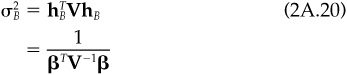
2. The variance of the characteristic portfolio ha is given by
3. The beta of all assets with respect to portfolio ha is equal to a:
4. Consider two attributes a and d with characteristic portfolios ha and hd. Let ad and da be, respectively, the exposure of portfolio hd to characteristic a and the exposure of portfolio ha to characteristic d. The covariance of the characteristic portfolios satisfies
5. If κ is a positive scalar, then the characteristic portfolio of κa is ha/κ. Because characteristic portfolios have unit exposure to the attribute, if we multiply the attribute by κ, we will need to divide the characteristic portfolio by κ to preserve unit exposure.
6. If characteristic a is a weighted combination of characteristics d and f, then the characteristic portfolio of a is a weighted combination of the characteristic portfolios of d and f; in particular, if a = κdd + κff, then
where
Proof We derive the holdings of the characteristic portfolio by solving the defining optimization problem The portfolio is minimum risk, given the constraint that its exposure to characteristic a equals 1. The first-order conditions for minimizing hTVh subject to the constraint hTa = 1 are
where θ is the Lagrange multiplier. Equation (2A.8) implies that h is proportional to V-1a, with proportionality constant θ. We can then use Eq. (2A.7) to solve for θ. The results are
and
This proves item 1.
We can verify item 2 using Eq. (2A.9) and the definition of portfolio variance. We can verify item 3 similarly, using the definition of β with respect to portfolio P as 
For item (4), note that
and
Items 5 and 6 simply follow from substituting the result in 3 and clearing up the debris.
Portfolio C Suppose
is the attribute. Every portfolio’s exposure to e  measures the extent of its investment. If eP = 1, then the portfolio is fully invested. Portfolio C, the characteristic portfolio for attribute e, is the minimum-risk fully invested portfolio:
Equation (2A.16) demonstrates that every asset has a beta of 1 with respect to C.9 In addition, for any portfolio P, we have
the covariance of any fully invested portfolio (eP = 1) with portfolio C is σ2C.
Portfolio B Suppose β is the attribute, where beta is defined by some benchmark portfolio B:
Then the benchmark is the characteristic portfolio of beta, i.e.,
So the benchmark is the minimum-risk portfolio with a beta of 1. This makes sense intuitively. All β = 1 portfolios have the same systematic risk. Since the benchmark has zero residual risk, it has the minimum total risk of all β = 1 portfolios.
Using item 4 of the proposition, we see that the relationship between portfolios Band C is
Portfolio q The expected excess returns f have portfolio q (discussed below) as their characteristic portfolio.
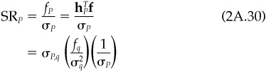
For any risky portfolio P (σP > 0), the Sharpe ratio is defined as the expected excess return on portfolio P, fP, divided by the risk of portfolio P:
Let q be the characteristic portfolio of the expected excess returns f:
Then
4. If ρP,q is the correlation between portfolios P and q, then
5. The fraction of q invested in risky assets is given by
Proof For any portfolio hP, the Sharpe ratio is SRP = fP/σP. For any positive constant κ, the portfolio with holdings κhP will also have a Sharpe ratio equal to SRP. Thus, in looking for the maximum Sharpe ratio, we can set the expected excess return to 1 and minimize risk. We then minimize hTVh subject to the constraint that hTf = 1. This is just the problem we solved to get hq, the characteristic portfolio of f.
Items 2 and 3 are just properties of the characteristic portfolio. For 4, premultiply 3 by hP and divide by σP. This yields
or
Part 5 follows from Eq. (2A.4):
Portfolio A Define alpha as α = f – β fB. Let hA be the characteristic portfolio for alpha, the minimum-risk portfolio with alpha of 100 percent. (Portfolio A will involve significant leverage.) According to Eq. (2A.5), we can express hA in terms of hB and hq. From Eq. (2A.4), we see that the relationship between alpha and beta is  . However, αB = 0 by construction, and so portfolios A and B are uncorrelated, and βA = 0.
In many cases, we will find it convenient to assume that there is a fully invested portfolio that explains expected excess returns. That will be the case if the expected excess return on portfolio C is positive. This is not an unreasonable assumption, and we will use it throughout the book. The next proposition details some of its consequences.
Proposition 3
Assume that fC > 0.
1. Portfolio q is net long:
Let portfolio Q be the characteristic portfolio of eqf. Portfolio Q is fully invested, with holdings hQ = hq/eq. In addition, SRQ = SRq, and for any portfolio P with a correlation ρPQwith portfolio Q, we have
Note that Eq. (2A.36) specifies exactly how portfolio Q “explains” expected returns.
4. If the benchmark is fully invested, eB = 1, then
Proof For part 1, note that  and fC > 0 imply eq > 0. From part 5 of proposition 1,
The holdings in portfolio Q are a positive multiple of the holdings in q, and so their Sharpe ratios and correlations with other portfolios are the same.
For item 2, start with  and use
  . This yields
  . If we multiply this by hQ, we get
  , and
, and  .
.
For item 3, premultiply Eq. (2A.27) by hB. This yields
and so
which gives 3.
For item 4, note that eB = 1 and  imply that
  . When this is combined with
  , we get 4.

We have built portfolios capturing the important characteristics for portfolio management. These portfolios will play significant roles as we further develop the theory. For example, if we want to build a portfolio based on our alphas, but with a beta of 1, full investment, and conforming to our preferences for risk and return, we will build a linear combination of portfolios A, B, and C.
Now focus on two characteristic fully invested portfolios: portfolio C and portfolio Q. At this point we would like to introduce a set of distinctive portfolios called the efficient frontier. Portfolio C and portfolio Q are both elements of this set. In fact, we will see that all efficient-frontier portfolios are weighted combinations of portfolio C and portfolio Q, so each element of the efficient-frontier is a characteristic portfolio. The return and risk characteristics of efficient frontier portfolios are simply parameterized in terms of the return and risk characteristics of portfolio C and portfolio Q.
A fully invested portfolio is efficient if it has minimum risk among all portfolios with the same expected return. Efficient frontier portfolios solve the minimization problem
subject to the full investment and expected excess return constraints (but not a long-only constraint):
We can solve this minimization problem to find:
where we have used the definitions of hC and hQ and have assumed that f ≠ e. So efficient frontier portfolios are weighted combinations of portfolio C and portfolio Q.
Remember that the correspondence between characteristics and portfolios is one-to-one. We can therefore solve for the characteristic aP that underlies each efficient portfolio, using Eq. (2A.45) and (2A.5). In each case, the characteristic is a linear combination of e and eqf, the characteristics underlying portfolios C and Q, respectively:
Figure 2A.1 The efficient frontier.
We can now use Eq. (2A.45) to solve for the variance of the efficient-frontier portfolios. We find
with
We depict this relationship in Fig. 2A.1. In this figure, portfolio Q has a volatility of 20 percent and an expected excess return of 7 percent. Portfolio C has a volatility of 12 percent and, therefore, an expected excess return of 2.52 percent. The risk-free asset appears at the origin.
We establish the CAPM in two steps. We have already accomplished step 1, showing in Eq. (2A.36) that the vector of asset expected excess returns is proportional to the vector of asset betas with respect to portfolio Q. In step 2, we show that certain assumptions lead us to the conclusion that portfolio Q is the market portfolio M, i.e., that the market portfolio M is indeed the portfolio with the highest ratio of expected excess return to risk among all fully invested portfolios.
If
■ All investors have mean/variance preferences.
■ All assets are included in the analysis.
■ All investors know the expected excess returns.
■ All investors agree on asset variances and covariances.
■ There are no transactions costs or taxes.
then portfolio Q is equal to portfolio M, and
Proof If all investors are free of transactions costs, have the same information, and choose portfolios in a mean/variance-efficient way, then each investor will choose a portfolio that is a mixture of Q and the risk-free portfolio F. That would place each investor somewhere along the line FQF’ in Fig. 2A.1. Portfolios from F to Q combine the risk-free portfolio (lending) and portfolio Q. Portfolios from Q to F’ represent a levered position (borrowing) in portfolio Q.
When we aggregate (add up, weighted by value invested) the portfolios of all investors, they must equal the market portfolio M, since the net supply of borrowing and lending must equal zero. The only way that the portfolios along FQF’ can aggregate to a fully invested portfolio is to have that aggregate equal Q. The aggregate must equal M, and the aggregate must equal Q. Therefore M = Q.
1. Show that  . Since portfolio C is the minimum-variance portfolio, this relationship implies that βC < 1, with βC = 1 only if the market is the minimum-variance portfolio.
2. Show that  ; i.e.,
  .
.
3. What is the “characteristic” associated with the MMI portfolio? How would you find it?
4. Prove that the fully invested portfolio that maximizes  has expected excess return f* = fC + 1/(2λκ).
5. Prove that portfolio Q is the optimal solution in Exercise 4 if  .
.
6. Suppose portfolio T is on the fully invested efficient frontier. Prove Eq. (2A.45), i.e., that there exists a ωT such that hT = ωThC + (1 – ωT)hQ.
7. If T is fully invested and efficient and T ≠ C, prove that there exists a fully invested efficient portfolio T* such that Cov{rT,rT*} = 0.
8. For any T ≠ C on the efficient frontier and any fully invested portfolio P, show that we can write

where T* is the fully invested efficient portfolio that is uncorrelated with T.
9. If P is any fully invested portfolio, and T is the efficient fully invested efficient portfolio with the same expected returns as P, μP = μT, we can always write the returns to P as rP = rC + {rT − rC} + {rP − rT}. Prove that these three components of return are uncorrelated. We can interpret the risks associated with these three components as the cost of full investment, Var{rC}; the cost of the extra expected return μP − μC, Var{rT − rC}; and the diversifiable cost, Var{rP − rT}.
For ease of calculation, focus on just MMI assets when considering these application exercises. The MMI is a share-weighted 20-stock index (you can consider it a portfolio with 100 shares of each stock). Also define the market as the capitalization-weighted MMI, or CAPMMI for short.
1. Restricting attention to MMI stocks, build the minimum-variance fully invested portfolio (portfolio C). What are the betas of the constituent stocks with respect to this portfolio? Verify Eq. (2A.16).
2. Build an efficient, fully invested portfolio with CAPM expected returns (proportional to betas with respect to the CAPMMI, which has an assumed expected excess return of 6 percent). Use a risk aversion of  , where
  is the risk of the CAPMMI.
a. What are the beta and expected return to the portfolio?
b. Compare this portfolio to the linear combination of portfolios c and B described in Eq. (2A.45). In this case, portfolio B is the CAPMMI.