Fun with Formulas and Functions

Maybe you won’t consider this chapter fun, exactly (although I do), but it should at least remove any stress accompanying your dealings with formulas and functions.

It starts with the two quick ways of accessing the most common spreadsheet functions (such as SUM and AVERAGE): the Function Button and the Quick Calculations Bar (which has an alternative identity as the Smart Cell View).

Then we’ll move on to creating your own formulas, starting with what you need to know about basic math operations as they relate to entering information in a formula: Typing Mathematical Operators and The Order of Operations. Next, we’ll make sure you understand Cell References—the different ways you can refer to cells; it’s particularly important to understand Relative vs. Absolute Cell References.

You’ll also learn how to work with The Formula Editor, building formulas and handling tokens inside in it, and then learn about Functions and Arguments—the built-in formulas that a spreadsheet can’t live without—and see how helpful The Function Browser can be.

The Function Button and Quick Calc Bar

The Function Button and the Quick Calculations bar provide very different approaches for quickly entering common spreadsheet functions—most of which provide handy statistics such as the average of a group of numbers, or the largest or smallest number in the group. Both approaches are quick and simple—no experience required.

Function Button

The most commonly used spreadsheet functions are available at the click of a button—the Formula button in the toolbar:

1. Select cells in a column or row that have numeric entries, making sure there’s a blank cell available after the selection.
2. Click the Formula button in the toolbar and choose a function from its menu.

Numbers enters the result of the function, such as the sum of the cells, in the cell beneath a column selection or to the right of a row selection. Behind the scenes, it has put a formula into the formula editor, using the function you chose from the menu and the cells you selected as its argument (Figure 88).

Figure 88: Using the Function button. Left to right: Selected cells, the Function menu, and the formula in the cell beneath the selection.

Note: Depending on your selection, you may see a cell range token (such as A2:A4) in the formula editor or, as in the figure above, a reference to the entire row, A.

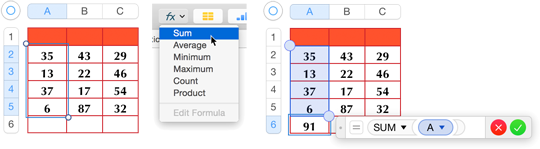
Here are some important things to note about this simple procedure. I use the SUM function as an example, but they apply to all choices in the Function menu:

• A formula OVERWRITES EXISTING DATA when it’s plopped into a cell, so make sure there’s a blank cell after the end of the selection.
• If you select an entire column or row with a click on its label, the formula is entered in the last cell, even if there are available blanks before it, and whether or not it’s defined as a footer row.
• If the entire column or row is filled with numbers, and you’ve selected all the cells, a new column or row is added to the table to accommodate the results.
• To sum several columns, select all the cells you want included and then choose from the Function menu. The results are inserted at the bottom of the selection, in each column.
• To sum several rows, select them by clicking or dragging across their labels (the numbers in the Row bar at the left of the table) so that Numbers knows you want to work with the rows in the block you’ve selected, and not the columns. Then choose from the Function menu.

Note: The SUM function is such a crutch in spreadsheets that if you open the formula editor in a cell and then simply drag across cells, it’s automatically entered in the formula. In related “adding is important” news: clicking or dragging on cells when the formula editor is open inserts an addition sign and the cell references.

All but one of the other functions in the Function button menu are straightforward:

• AVERAGE: The AVERAGE function provides what we usually refer to as an “average,” but more properly, it’s the arithmetic mean (and that’s pronounced arithMETic). The related MEDIAN and MODE functions are available when you’re working in the formula editor.
• MINIMUM and MAXIMUM: These find the smallest and largest values in a range of cells.
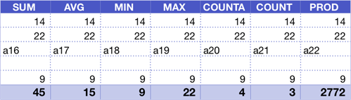
• COUNT (COUNTA): This is the problem child in the family. The menu lists the COUNT function, but in fact it’s the COUNTA function that’s entered into the cell, as you’ll see if you check the cell’s formula afterward. It’s beyond my imagination (and, like Han Solo, “…I can imagine quite a bit”) why it’s listed this way, especially as it’s correctly defined as COUNTA in the Quick Calc bar.

  The COUNTA function counts how many cells in its referenced range are not blank (think of it as COUNTA for data). COUNT, on the other hand, counts cells that contain numbers, expressions that resolve to numbers, or dates, ignoring both blanks and any other kind of data, such as text (Figure 89).

Figure 89: The bottom row shows the effect of each of the Function button’s available functions, as well as the standard COUNT function, for comparison to COUNTA.

• PRODUCT: The only non-statistical function in the menu, this multiplies the selected cells together using the PRODUCT function instead of mathematical operators. So, you wind up with PRODUCT(B1:D1) instead of B1 × C1 × D1.

Quick Calculations Bar

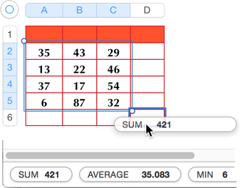
At first, I thought the Quick Calc bar at the bottom of the Numbers window was just a quick reference—you’d get an immediate idea of the sum, average, and so on, of any cells you select. Which, of course, you do, and that’s a convenience even if it went no further.

But then I wondered… and, yep, by golly, drag one of the statistical tokens into any cell in a table, and the appropriate formula, calculated from whatever’s selected in the table, is entered in that cell, no matter where you drop the token (Figure 90). And there’s the big difference between using the Function button and the Quick Calc bar: with the former, the formula is entered in a blank cell adjacent to the selection, while dragging from the latter lets you place the formula anywhere.

Figure 90: Drag a token from the Quick Calc bar and drop it anywhere in the table to create a formula for that function.

The Quick Calc bar starts out with tokens for five of the six functions in the Function button (PRODUCT is missing), but you can customize it:

• Add a token: Add other functions by selecting them from the more than two dozen listed in the Action pop-up menu at the far right of the bar (Figure 91).

Figure 91: Use the Action menu to add more tokens, and when your bar runneth over, click the scroll arrows to get to other tokens.

• Reorder the tokens: Drag them to their new positions.
• Remove a token: Uncheck it in the Action pop-up menu.
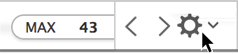
• Scroll the overflow: When your token collection no longer fits in displayed area of the bar, scroll it by clicking in the arrows at its right end (shown in the figure above), or use a two-finger swipe on a trackpad.

Smart Cell View

When a single cell is selected, the Quick Calc bar morphs into the Smart Cell View, which displays the underlying contents of a cell. This is very convenient in many circumstances:

• When a cell is formatted to display, for example, a number to the second decimal place, the Smart Cell View shows the fifteen-decimal-place, actual number stored there.
• While a cell displays the results of a formula, the Smart Cell View shows the formula itself.
• When a formula-error warning takes over a cell, a click on the cell describes the error, while the Smart Cell View shows the formula.
• If the formula editor is open for a cell, its result is shown in the Smart Cell View—this is helpful because an open formula editor blocks your view of the cell, and moving it can be inconvenient.
• A corollary to the last item: the results of the formula are displayed as you enter it. So, you can track a complicated formula as you build it.

Formula-building Basics

You may be eager to get to the actual formula-building part of working in the formula editor, but first there are some fundamentals to cover.

Typing Mathematical Operators

To enter formulas, you need to know basic computer-math conventions for typing multiplication and division, and other math symbols.

But first, a reminder: before you type even a simple formula like 1+1 into a cell, you must start with an equals sign to tell Numbers that it’s a formula and not a string of numbers and symbols that might stand for, say, a serial number. As soon as you type the equals sign, the formula editor pops open. Just keep typing; edit, if necessary, within the editor, and click Accept or Cancel when you’re finished. (I have lots more to say about the formula editor later, when it comes to working with functions.)

To enter basic mathematical operators in the editor:

• Addition and subtraction: Type the standard plus and minus signs.
• Multiplication and division: The asterisk (Shift-8) has long served as the multiplication symbol on computers, while the forward slash (/) is used for division. But Numbers is elegant in this regard: type either of those symbols in the formula editor, and they are automatically transformed to genuine multiplication and division symbols when you close and reopen the editor. So, type 3*4/8 and you’ll get 3×4÷8.
• Exponents: Type the caret (^) in front of the exponent: 6^3.

The Order of Operations

When you construct a formula that includes multiple mathematical operators, some operators take precedence over others, so the numbers aren’t always handled from left to right. (This hierarchy, or order of operations, is not specific to Numbers or spreadsheets, but a math basic.)

Multiplication and division are of equal importance, but are performed before addition and subtraction (which are of equal importance to each other). Reading from left to right might lead you to believe that 22-8÷2 is the same as 14÷2 but that’s incorrect: with division taking precedence over subtraction, it boils down to 22-4.

You can override the normal order of operations with parentheses; items inside parentheses are always performed first. So:

22-8÷2 = 22-4 = 18

but

(22-8)÷2 = 14÷2 = 7

Cell References

The basic cell name is its column and row—in effect, its coordinates: B5, K9, AB14. (After Z, columns have double letters: AA, AB, and so on.) But, cell references are often much more complex. In this topic, I tell you about several types of references:

• Referencing multiple cells, in groups such as an entire row or column, by coordinates, and single or multiple cells in another table or on another sheet (just ahead)
• Using written out names to refer to cells (see Referencing by Header Names)
• Creating a cell reference that won’t change when a formula is copied (in Relative vs. Absolute Cell References)

Cell Coordinates

You’ll usually enter cell references in a formula by clicking in, or dragging across, table cells. Still, you need to know about the many ways to refer to cells because sometimes you will want to type them, but also because Numbers enters these reference when you click and drag the targets, and you’ll want to be able to read them in a formula. Here’s what references can look like:

• Single cell: Its column and row: A1 or B247.
• Range: Its upper-left and lower-right cells: B2:B12 or A1:AF247.
• Entire row: The row number twice, with a colon in between: 2:2.
• Multiple entire rows: The first and last row numbers, separated by a colon: 2:4 or 15:32.
• Entire column: The column letter: B.
• Multiple entire columns: The first and last column letters, separated by a colon: B:D.

Note: When you reference full rows or columns in a formula, the contents of header and footer cells are ignored.

• Cell or range in another table on the same sheet: The table name, followed by double colons and the cell reference: TableName::B5 or Personal::B5:J12.
• Cell or range in another table on a different sheet (tab): The sheet name, the table name, and the cell coordinates, with double colons between the elements: SheetName::TableName::B5 or Expenses::Personal::B5:K9. You can’t reference a cell in a different document.

Referencing by Header Names

You can make your formulas easier to read by referring to them by row and column header names instead of row coordinates. To set this up, choose Numbers > Preferences > General and check Use Header Names as Labels. And then set up row and column headers—not just labels for your data, but defined row and column headers, as described in Headers and Footers.

With this setup, the formula editor uses cell references like January:Income or Q1 Profit instead of C:20. If you type C:20 into the formula editor, or click the cell to enter a reference, the formula editor substitutes the header names. As a bonus, if you start typing a header name in the editor, you’ll get an autocomplete suggestion for any matches.

Note: You can’t mix a header name with a row or column coordinate, such as Budget:3 for the third row in the column labeled Budget.

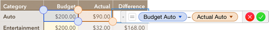
Figure 92 shows a slice from the Personal Budget template that uses header references instead of cell coordinates; you can see how much clearer the formula is than if it referred to B2-C2.

Figure 92: Header names instead of cell coordinates in a formula make it easier to construct and read.

Here’s how to refer to cells by header names:

• Single cell: Give the header names for the column and row, citing the column first. In the previous figure, that’s Budget Auto, not Auto Budget, instead of B2.
• Entire row or column: Use the header name instead of the row number or column letter: Auto, Entertainment, Budget, Actual.
• Cells, rows, or columns in another table or sheet: If the cell name, based on its row and/or column header, is unique to the document (that includes all the tables in all the tabs), you can refer to it by just its name: Budget Auto. Otherwise, first identify the table or sheet followed by a double colon and then the named cell reference: Summary by Category::Budget Auto. Usually, you’ll enter such a reference by clicking in the other table so you don’t have to think about capitalization. If you type it, however, you can ignore capitalization and Numbers will correct it for you when you enter the formula. Spelling and spaces, on the other hand, must be exact, or you’ll get a formula error.

Relative vs. Absolute Cell References

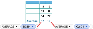
If you set up a function that averages the numbers in a column—AVERAGE(B2:B4), say—and then copy or autofill it to another column, the function’s argument changes to accommodate the move; it refers to different, analogous cells, such as AVERAGE(C2:C4) (Figure 93). This is called relative cell referencing, since the changes keep the referenced cells relative to the formula’s cell. In effect, this copied formula really says “average the three cells above me.”

Figure 93: When the formula in B5 is copied to C5, the cell references automatically change to keep them relative to the formula’s cell.

Note: Automatic relative cell referencing works when you paste or autofill but not when you move cells by dragging them (Moving Data within a Table). Moving a cell leaves the contents exactly as you entered them.

But sometimes relative cell referencing isn’t helpful. Say you have to convert from kilometers to miles, so you put the conversion factor (0.6214) in a cell and refer to it in a formula. When you copy the formula down, you get errors because the default relative referencing refers to empty cells (Figure 94).

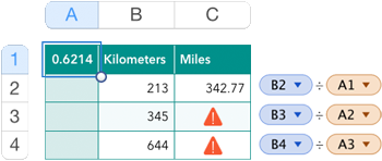
Figure 94: The formula in C2 works fine in its row, but when it’s copied down, the references to A1 change to refer to empty cells.

To avoid that problem, formulas can use absolute cell referencing, which means the cell references don’t change when you copy or autofill the formula. Absolute references are indicated by using a dollar sign in front of the row or column reference (or both); an absolute reference to cell A1 in the previous figure would be $A$1. In a situation where you want the column reference to remain static but the row to change, you’d use $A1; for the reverse, you’d use A$1.

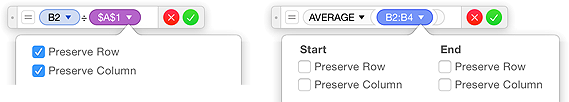
You can type the dollar signs, or use the popover menu from a cell token in the formula editor (Figure 95). Check Preserve Row or Preserve Column, or both; you’ll see the dollar signs inserted into the cell reference. (Tokens and their menus are covered in detail ahead, in Cell References and Tokens.)

Figure 95: Left: A cell reference token’s popover lets you set absolute references. Right: A range token provides absolute reference choices for each extreme of the range.

Note: If you’re using header names instead of row/column references, insert the dollar sign in front of either or both names: $Budget Auto or Budget $Auto or $Budget $Auto.

Tip: You can use keyboard commands to change relative and absolute referencing for a selected token. Press Command-K and Command-Shift-K to cycle through the options for a cell token. For a range token, use Command-Option-K and Command-Option-Shift-K.

The Formula Editor

There’s quite a lot to know about working in the formula editor efficiently, and this section provides the details. But let’s start with a quick look at how to get in and out of the formula editor:

1. Select a cell and type an equals sign to open the formula editor. (If you type an equals sign and it appears in the cell, that cell is specifically formatted for text. In the Format Inspector’s Cell pane, choose Automatic from the Data Format menu to make the cell recognize the signal for the formula editor.)
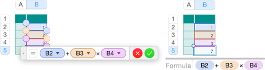
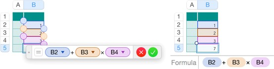
2. Click or type your way to the formula you need. For example, your formula could read 1+1 or B2+B3×B4. Numbers changes cell references to tokens, as you can see in the figure below; I talk more about them a little later.
3. Close the formula editor by clicking the Accept button or pressing Tab or Return to move to the next cell. (Remain in the cell by pressing Enter or Command-Return). To cancel your entry or edits, click the Cancel button or press Esc.

To re-open the formula editor, double-click the cell, or select the cell and press Option-Return.

A cell displays the results of a formula, but you can see the formula that’s stored in a selected cell in the Smart Cell View at the bottom of the window (Figure 96).

Figure 96: Left: The formula editor open in B5. Right: With B5 selected, the Smart Cell View shows the formula.

Move or Resize the Editor

The editor is easy to move, which is a good thing, since it obscures its own and adjacent cells. Just place your pointer over the editor’s left edge until it changes to the grabber hand, and drag it.

It’s not obvious that you can resize the editor, especially since it automatically expands horizontally as a formula gets longer. To change the length or height, hover over either the bottom or right edge for a resize cursor and drag. To change both dimensions at once, hover over any corner until you see the pointing hand and drag (Figure 97).

Figure 97: Left: Drag the formula editor to any position. Right: Resizing from a corner; note the gray scrollbar that indicates not all of the formula is currently showing.

If you click a sheet tab when the formula editor is open, the editor stays floating on the screen, even when you’ve switched to another tab. This makes it easy to enter a reference to a cell in a far-off table with a simple click. You won’t have to remember the sheet, table, and cell name on one sheet—and the syntax for all of that info—to enter it in a formula on another sheet.

Cell References and Tokens

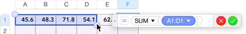
To enter cell references in the formula editor, click a cell, drag across multiple cells, or simply type (B12, for instance). The formula editor turns the reference into a token.

Numbers assigns each token a color in the editor; the token’s related cell is highlighted with that color, making it much easier to analyze the components of the formula. In addition, when the formula cell is merely selected, its referenced cells are colored both in the table and in the formula displayed in the Smart Cell View (Figure 98).

Figure 98: Left: When the editor is open, the cells’ colors match their tokens. Right: A selected formula cell has color-keyed cells in the table and tokens in the Smart Cell View at the bottom of the window.

To change the cell reference at any point, click its token, which darkens in response, and then:

• Replace it: Click a cell, drag across multiple cells, or simply type.
• Edit it: Drag the blue handles at the corners of the selection in the table to add or remove cells (Figure 99).

Figure 99: With the token selected, you can change a cell-range reference by dragging a selection handle.

• Move it: If the cell range is going to be the same size, but shifted (changing from A1:D1 to B1:E1, for instance), you can drag the selection itself—not with the handles, but from within the highlighted area—to a new position.

You can also use the Option and arrow keys, with and without Shift, to enter and edit cell references. I discovered this accidentally, and am not quite sure how handy it will be in the long run. There are two approaches:

• For a selected token: Press Option and an arrow key to move the highlight that shows referenced cells in the table. If for instance, your token refers to C8 and you press Option-Down arrow, the token changes to C9. If the token is for the range B2:B8, pressing Option-Right arrow changes it to C2:C8.

  Add Shift to expand the size of the cell reference range instead of moving it. If the token is for C8, Option-Shift-Down arrow changes it to C8:C9.

• For a new cell reference in the formula: When the blinking insertion point is in the formula (click in a spot, or press the Left or Right arrow key to deselect a token and place the insertion point), press Option to see a cell-reference token whose color varies depending on the color of any nearby tokens. With Option still down, press an arrow key to get a cell reference to a cell adjacent to the currently selected one.

  Add the Shift key, and your selection expands in the direction of the arrow key you’re using.

Note: Using cell token pop-up menus was covered previously, in Relative vs. Absolute Cell References.

Function and Argument Tokens

Cell references aren’t the only tokens in the formula editor. Functions and Arguments are represented by tokens, too.

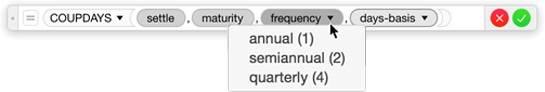
When you enter a function that needs arguments, the formula editor prompts you with a token for each one. If the argument uses something like a number code to represent an option, its menu helpfully provides a cheat sheet (Figure 100).

Figure 100: Each argument for COUPDAYS is represented by a token. The frequency menu tells you which numbers the function accepts as a frequency parameter, and what they stand for.

Tip: To select the next or previous argument token, you can press Tab or Shift-Tab. (This doesn’t work for other types of tokens.)

Enter and Edit Functions from the Keyboard

Are you a keyboard jockey? You can enter all of the information you need in a formula without leaving the keyboard.

The formula editor tries to read your mind as you enter information, popping up suggestions as you type. You can click on a suggestion, but you can also select it with keystrokes. And, since a selected token can be replaced by typing, and you can move between argument tokens by pressing Tab and Shift-Tab… you get the idea. Try this procedure to familiarize yourself with the click-free way to enter formulas:

1. With a cell selected, type an equals sign to open the formula editor.
2. Type ran. As you type r, Numbers suggests the nearest alphabetic equivalent, RADIANS, inside the token, and displays a bar showing other functions that begin with those letters. When you get to n, RAND is suggested in formula editor, and the bar beneath it narrows to include only functions that begin with ran.

   Tip: In case you didn’t notice: functions are displayed in uppercase letters in their tokens, but you can type in lowercase.

3. Hit Tab to move to the bar; the selection jumps to RANDBETWEEN in the bar, because you’ve already declined to use the first item, RAND. (If you tab again, you’ll move to the next item in the bar, which might be displayed partially, or not at all; if you tab beyond the last choice, it cycles back to the first one.)
4. Press Return to enter the RANDBETWEEN selection; the bar disappears, and the function editor displays the function and its argument tokens (Figure 101). The first argument is already selected; type a number to replace it. Press Tab to move to the next token and then type another number.

   

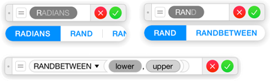
   Figure 101: Top: Typing R supplies many suggestions, but by the time you type RAN, the choices narrow and you can use Tab to select RANDBETWEEN. Bottom: When the function is in the editor, you can tab from one token to another.

5. Press Command-Return to close the formula editor.

The Clairvoyant Formula Editor

The formula editor always tries to predict what you’re typing, and shows its best guess in the current token. If it has read your mind correctly, you can press Return to accept the token and move on to your next action.

This clairvoyance is applied to every token in the formula editor, not just function tokens. Sometimes this is a great help. But other times the editor is like an overeager puppy, doing anything it can to get your attention and then tripping over its own feet. When, for instance, you intend to type the cell range B2:B4, when you type B you’ll get suggestions for not only cells in column B, but also anything else that begins with B that just might be what you want as a cell reference—including any header with text that starts with B, any table (on any sheet) whose name begins with B, and any sheet tab that starts with B. Just keep typing until the puppy calms down.

Work with Text in the Formula Editor

Sometimes it’s easier to work with text in the formula editor rather than with its tokens. Say, for instance, you entered a cell reference for something on another sheet: do you really want to go to the other sheet and reselect the area when all you need is to change B2:B7 to B2:B8? Or scroll through the Function Browser to replace a function token when you just need to change HLOOKUP to VLOOKUP?

You can change a single token, or the entire formula, to text:

• Change a token: Double-click the token.
• Change the entire formula: Open the function token menu and choose Convert Formula to Text (Figure 102). (Choosing Convert Function to Text is the same as double-clicking the function; Show in Function Browser is covered later, in The Function Browser.)

Figure 102: Use the function token menu to make the formula editor display editable text.

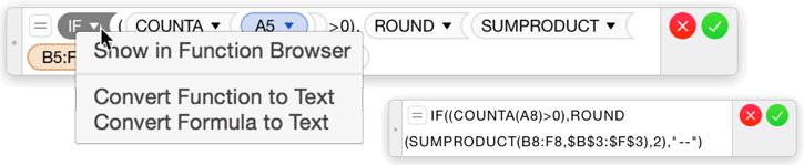
To return to the token view, close the formula editor and reopen it. You can do this quickly with the keyboard: press Enter or Command-Return to close the editor but remain in the cell, and then press Option-Return to open the editor again.

Tip: When you’re working in text, you can make things more readable by adding extra spaces to delineate pairs of nested parentheses.

Error Reports

If you’ve made a mistake when constructing a formula or with a function, the cell displays an error symbol (Figure 103). Click it to get at least a clue as to what you did wrong. Some explanations, such as “There is a syntax error,” are less helpful than others.

Figure 103: Click the error symbol to see an error report.

Because the cell is selected when you look at the warning, the formula stored there is helpfully displayed in the Smart Cell View at the bottom of the window.

Functions and Arguments

A function is a built-in formula that spares you from reinventing the wheel when you perform mathematical (or text-based) operations. Calculating an average, for instance, requires adding up a series of numbers, and then dividing that sum by how many numbers you added together. In spreadsheet-speak, that formula might look like this: (A1+B1+C1) / 3. But, instead of typing all that (taking time and risking errors), you can use a function—AVERAGE—that knows to add things together and then do the division.

You tell the function which numbers to use by providing one or more arguments in parentheses. If the argument refers to cells containing numbers, the reference could be a cell range AVERAGE(A1:C1) or a list AVERAGE(A1,B1,C1). Some functions need, or can use, specific numbers rather than cell references as arguments. These are sometimes referred to as constants because… duh… they don’t change, while references can change when cell contents change. So, you could actually use a formula like this: AVERAGE(12,14,18).

Functions have very specific needs, and you must use the correct syntax—the grammar of functions—or they won’t work. For instance, you can’t simply say B1 OR C1; you must use OR(B2,C1). But you don’t have to worry about remembering the correct syntax for hundreds of functions. As you saw in the previous section, when you enter a function in the formula editor, it comes with tokens that stand for each of its arguments, with the proper syntax already in place.

Nested Functions

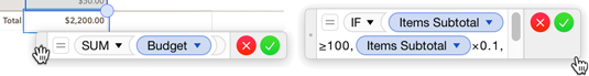
It’s not unusual to use more than one function in a formula: =SUM(A2:A27) + RANDBETWEEN(2,10) for instance. What’s slightly less usual, but potentially very confusing, is the use of nested functions—one function inside another, with the inner one replacing an argument the main function needs.

In an example elsewhere in this book, there’s a small table that calculates whether a customer gets a discount, which happens when one purchased item is over $40 or the total order is more than $100. Cell B5 holds the total order with SUM(B2:B4); cell C2 checks for the highest-priced item with MAX(B2:B4). The discount calculation checks if B5 is over $100 or C2 is over $40. The part of the formula that checks whether either discount threshold is met uses the OR function and references the cells holding the calculations:

OR (B5>100, C2>40)

It’s unnecessary to do this two-step process, however, because the calculations themselves can go directly in the OR construct. This is the same formula snippet as the one above, with the cell references replaced by the formulas:

OR (SUM(B2:B4)>100, MAX(B2:B4)>40)

In the real world, these nested functions would be further nested in the fuller formula, which uses the IF function to describe the results if either of these formulas is true, but there’s no reason to go there now—you get the picture.

Mind Your Parentheses

Numbers bends over backwards to help you parse function components by displaying the function name in an odd shape that serves as part of an opening parenthesis; the closing parenthesis a matching chunky moon-slice.

When there’s more than one set of parentheses in a formula, you can click on any parenthesis to highlight its partner, and all the tokens in between, to help you analyze the elements and how they go together (Figure 104).

Figure 104: Top: The formula editor as it opens. Center and bottom: Click one parenthesis to select its partner and interior tokens.

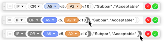
If you’re typing or editing a function with parentheses, you can just type them regularly and they’ll be replaced with their graphical representations. And, you can skip typing a final closing parenthesis completely; Numbers inserts it for you. (By “final,” I mean the last one in the formula, not the closing parenthesis for any interior component.)

The Function Browser

The Function Browser replaces the Format Inspector in the panel at the right of the window the moment you type an equals sign to start a formula or otherwise open the formula editor. The Sort & Filter Inspector, however, holds its ground under these circumstances, so to see the Function browser you must either choose Show Function Browser from a function token menu or—in another interface oddity—click the Format Inspector button.

The Browser’s upper area lists categories and functions. Beneath that is description of the selected function (Figure 105).

Figure 105: The Function Browser’s upper area shows categories and specific functions. Select an item in the list to get its description, syntax, and details.

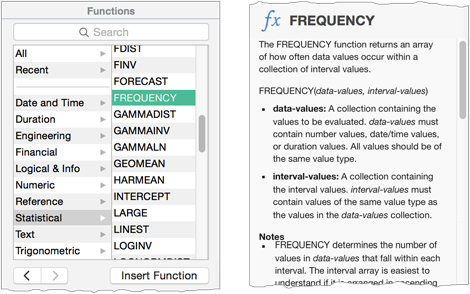
To use the Function Browser:

• Select a function to see its description and syntax in the lower part of the Browser.
• Use the search field at the top of the Browser to jump directly to the function you want.
• Click the Previous and Next arrow buttons under the list to review functions you’ve previously selected.
• Put a selected function into the formula editor by clicking the Insert Function button.
• Insert any function by double-clicking its name in the list.