Data Input

Put data in a cell? Sure, just click in a cell and type—what else is there to know? Well, there’s the many different Types of Data that Numbers recognizes, how to make sure it knows which you’re entering, and how Text Wrap in Cells works when your cell runneth over.

And then there’s letting Numbers do more of the work for you with Autocomplete and Autofill. You can also do more than just copy and paste data with Copy and Paste; you can leave the cells’ formatting behind if you want, for instance, or paste only the formatting in the new location.

There’s also Numbers’ very Special Data-input Formats that both speed data entry and ensure accuracy: Checkboxes, Star Ratings, Pop-up Menus, and Sliders and Steppers.

Data Entry Basics

To enter data, click a cell to select it and type. This is convenient—you don’t have to click a second time to put the blinking insertion point in the cell before you type, but it can also be dangerous because it’s so easy to mistakenly type over existing data. If you want to edit in a specific spot in a cell that’s not selected, double-click at that spot; the first click selects the cell, and the second one places the insertion point.

Each cell is like a teeny-tiny word processor. This means, for instance, that you can double-click to select a word or drag across characters to select them when you want to edit a selected cell’s contents.

You have to let Numbers know that you’ve finished your input before it can calculate formulas or do its auto-formatting tricks. For that, go to another cell, or press Command-Return to deselect the contents but remain in the current cell.

To erase all data from a cell, select the cell and press Delete. This works for a selected range of cells, too, so you can clear multiple cells with a single keypress. Cell formatting, including text formatting, remains “attached” to the cell; comments are removed.

Tip: To return a cell to its pristine non-formatted condition when deleting its data, choose Edit >Clear All.

Moving Data within a Table

To move a cell, select it and then “press” (click-and-hold) the cell until it looks like it’s lifting from the table. Drag it to another spot and drop it there (Figure 41); the cell formatting comes along for the ride. You can do the same with multiple selected cells, too.

Figure 41: Left to right: Select the cell; press the cell until it lifts up; drop it in the new location.

But be careful! If you drop the cell on top of a cell that has something in it, the existing contents are replaced.

You can also drag some or all of the text in one cell to another cell, similar to how you can move text in a word processor: select it and then drag it to the new spot. The text formatting comes along with it, but not the cell formatting, since the cell itself wasn’t selected. However, as with moving a cell, the text you drag will wipe out the contents of the target cell.

Types of Data

For a cell that you’ve left with the default Automatic data format setting in the Format Inspector’s Cell pane, Numbers automatically recognizes most data types:

• Number: When you finish entering a number, it’s automatically right-aligned in the cell to reassure you that it’s been recognized as a number.
• Text: Text is anything that doesn’t qualify as any of the other data types, so it includes pure text as well as mixtures of text, numbers, and/or symbols. Text is automatically left-aligned in a cell.

  Month names, however, are assumed to be labels for adjacent cells, and are automatically right aligned. Numbers also conveniently expands month abbreviations automatically, so you can type Jan, and it turns into January as you leave the cell.

• Formula: Typing an equals sign (=) indicates you’re entering a formula.
• Date/Time: You can’t have a date without a time, or a time without a date. (Mind bender: a date is actually a time.) Type 5/23 and you see that in the cell, but what’s stored is 5/23/[current year],12:00:00 AM. Conversely, enter a time like 12:27 and it’s [current date], 12:27:00 PM that’s stored. The cell defaults to displaying only the part of the date/time that you entered. Simple month-name entries also include a full date (the first of the month, with the current year) and 12:00 AM.
• Duration: The duration units are week, day, hour, minute, second, and millisecond. Numbers assumes the most common durations are the ones you want, so entering 2:3:4 in a cell is understood as 2h 3m 4s (and therefore a time—2:03:04 a.m.), not 2d 3h 4m.

Translating Time and Duration Entries

If you don’t format a cell specifically for a time or date (see Data Formats), when you type 1:2 or 1:2:3 Numbers interprets them as times: 2 minutes after one o’clock in the first example, 2 minutes, 3 seconds after one o’clock in the second. Four digits with colons is always a duration: 1:2:3:4 is 1 day, 2 hours, 3 minutes, 4 seconds. Use five digits—1:2:3:4:5—and Numbers interprets the first digit as the number of weeks.

You can enter dates and durations with signifiers so Numbers knows what you mean. Override the “two or three digits is a time” approach by typing 1d2h3m, and Numbers separates the entry into the default duration format 1d 2h 3m. And, when you use signifiers, you can even skip some time or duration units and Numbers will fill in the blanks: type 4h27s and you’ll get 4h 0m 27s.

If a cell is formatted to hold a duration, however, you don’t need signifiers; you can simply type one, two, or three numbers separated by colons.

(Note that if you type 14d, it gets translated to 2w as soon as you enter the data; similar translations occur when you provide a surfeit of any unit.)

Graphics Are Not Data

It seems that you can put an image in a cell: with an image on the Clipboard and a cell selected, choose Edit > Paste and a tiny version of the image winds up in the cell. You can even paste in a video or audio file and its associated image will be stored in the cell. But the image is strictly background fill: data appears on top of it. (Now that I’ve let that particular cat out of the bag, I’m counting on you to not overdo it.)

The image is no longer an independent entity—you can’t drag or copy it out of the cell. That’s because it’s not data any more; it’s just formatting, like color—which is why your cell data goes on top of it.

If you mistakenly paste an image into a cell, it’s not obvious how to get rid of it—unless you remember that it’s just a cell format at that point, not an actual image. Simply select the cell and, in the Format Inspector’s Cell pane, choose No Fill.

Text Wrap in Cells

When you type too much text in a cell, it wraps inside the confines of the cell, changing the cell’s height as necessary. This is controlled by a setting in the Format Inspector’s Text pane: in the Alignment section, Wrap Text in Cell is checked by default.

As you can see in Figure 42, long words in a narrow cell are broken where necessary, irrespective of proper hyphenation.

Figure 42: With text wrap, the text breaks into separate lines in a narrow cell, and words may be broken apart irrespective of syllabification.

Tip: To insert a line break and force something to the next line of text inside a cell, press Option-Return.

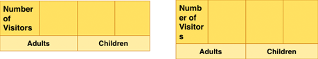
When you turn off Wrap Text in Cell for selected cells and then type too much text, the words continue merrily on their way into the next cell if it’s empty, and even into the following cells if necessary. This is a convenience when you’re creating multi-column headings because you won’t have to merge cells to span the columns. If the next cell is occupied, all the text you type is stored in the first cell, but you won’t see the overflow unless the cell is selected.

Letting text spill over into adjacent cells can be convenient, but there are formatting advantages to merging cells purposely (see Merge and Unmerge Cells) rather than letting the spillover do it for you, as you can see in Figure 43.

Figure 43: Left: Original cells. Center: Text “spillover” when text wrap is inactive. Right: Text entered in merged cells, and formatted to be centered over the two columns beneath it.

Autocomplete

Try it: The 3·Autocomplete States sheet in The Hands-on Example Spreadsheet has a list of states that begin with N so you can experiment with the Autocomplete feature.

Make it: List several states in a column, including New Jersey and several others that begin with New, a few that start with N but not New, and some that start with a different letter.

To turn on Autocomplete, choose Numbers > Preferences > General and then, under Editing, check Show Suggestions When Editing Table Cells.

This is not the infamous autocorrect that sends messages saying you’ll be late because you haven’t finished eating your kids for lunch. Autocomplete works smoothly and both saves time and ensures accuracy: when you start typing text in a cell, it provides a pop-up of matching contents elsewhere (above or below) in the column (Figure 44).

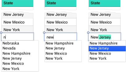
Figure 44: Left: Typing n triggers a list of entries beginning with N. Center: While ne kept Nebraska and Nevada in the list, with new, the list is down to four states. Right: Adding a space and j suggests New Jersey; arrow down to New Jersey to see Jersey selected in the cell. If you keep typing, it will be overwritten.

Tip: You can type in lowercase and Numbers still finds, and enters, a capped version of the text if that’s what’s in the list, as you can see in the figure above.

Continue typing to narrow the list—or to make an entirely new entry, of course—or select from the list by clicking the item you want. Or, press the Up and Down arrow keys to move in the list (or Tab to cycle through it) and when your target is highlighted, press Return to place it in the cell.

Autofill

I love autofill—and so will you once you see its versatility. It is, in effect, a smart-copy feature that figures out what to put in cells when you drag the autofill handle from a selected cell, or cells, in any direction. It can simply repeat the same information (handier than you might think), or recognize a pattern and continue it int0 other cells. It’s an incredible timesaver.

Warning! When you use autofill, it overwrites data in the cells you copy into, and you get no warning (other than this one). As usual, Edit > Undo is your friend.

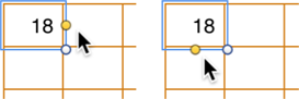
To use autofill, select one or more cells (even a complete row or column), hover near the midpoint of any side of the selection, and drag the yellow autofill handle (Figure 45) across the cells you need filled.

Figure 45: When you hover near the edge of a selected cell or group of cells, the yellow autofill handle appears at the midpoint.

As an alternative to dragging the autofill handle, you can select the cells where you want the data to go, with the source cell as the first or last cell in the selection, and then use the Table > Autofill Cells submenu, choosing Right, Left, Up, or Down.

Before we move on to details about autofilling, here are some basics to keep in mind:

• Autofill down or to the right, and the data increments; fill up or to the left, and it decrements, moving into negative numbers if necessary.
• Data formats (dollar signs or the number of decimal points displayed, for instance) are included in the autofill.
• Some cell formats (background fill) are copied to the autofilled cells; others (borders) are not.
• Comments attached to cells are not copied.
• A merged cell can’t be part of an autofill—either as the originating or a receiving cell.

Tip: When you drag for an autofill, Numbers doesn’t let you drag into headers or footers from body cells—a clever blockade for sloppy drags. However, you can use autofill within headers or footers, a convenient feature when you need to repeat a pattern of subheader information beneath merged header cells.

Start with a Single Cell

When you select only a single cell to start the autofill process, its contents populate the other cells. Whether the cells are filled with identical or altered data depends on what’s in the original cell:

• Simple data: Plain text (that is, not mixed with a number that might indicate a pattern) and numbers are copied into the new cells. A single letter of the alphabet, however, is treated as the beginning of a sequence.
• Formulas: A formula is copied into new cells with automatic changes so that cell references inside each formula will be relative to the new cell. If you’re not familiar with this concept, or wish to override it, see Relative vs. Absolute Cell References.
• Sequence triggers: If you start with a single cell containing data that Numbers thinks is the first of a sequence, it fills the new cells with the patterned data. These are sequence triggers:
  • A single letter.
  • A day of the week (a full or partial name).
  • A month name.
  • A date or time (such as 12:15).
  • A number appended to some text. The text remains static while the number changes: Sample 1 autofills to Sample 2, Sample 3, and so on. Even Sample1, with no space or other delimiter, works as a trigger.

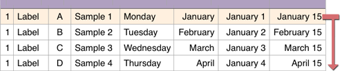
You can do multiple autofills at once. Figure 46 shows the result of selecting cells in a row and autofilling all of them downward.

Figure 46: All these columns were autofilled from the top row with a single drag. Note the first two columns were simply copied as is, since they had nothing that indicated a pattern.

Try it: You can try autofill sequence triggers from single cells in the 4·Autofilling sheet of The Hands-on Example Spreadsheet.

Start with Multiple Cells

You can use multiple-cell autofill in three ways: to repeat the contents of the selected cells, to define a pattern for a fill, and to override what might otherwise be interpreted as a pattern.

Repeat the Cell Contents

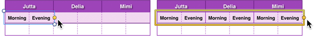
Say you have data that tracks mental acuity stats in the morning and the evening for each person in a study. The people’s names are in a header row, and a subheader row contains the Morning and Evening labels for each person. You can fill in the subheaders for the first person, and then select them and drag the autofill handle to the right to fill in the rest of the row with the pair of labels (Figure 47).

Figure 47: Autofilling can start with multiple cells.

Define a Pattern

While certain entries trigger a pattern autofill from a single selected cell, as described previously, you can define all sorts of patterns by creating “sample cells,” and autofilling from them. Two cells can easily define a pattern for autofill:

• Odd or even numbers: Fill adjacent cells with 1 and 3, or 2 and 4.
• Other number patterns: Start with a recognizable pattern such as 5 and 10, 10 and 20, or 100 and 125. If you need weird letter patterns, you can do the same thing: start with A and C, or A and G, for instance.
• Alternate days of the week: Start with Monday and Wednesday, or any pair with a skipped day. (This can be handy to schedule shifts for carbon-based life forms.)
• Specific days of the month: Use January 1 and February 1, or January 15 and February 15, or any two consecutive months with specific days.
• Reversed lists: Need a countdown from 100 to 1? From February 28 to February 1? Just enter the highest value in the cell where you need it and put the next value in the following cell; select them both, and your downward autofill will continue the reversed list.

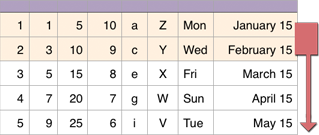
Figure 48 shows various multiple-cell patterns used as the basis for autofill sequences.

Figure 48: For each of these columns, the autofill started with the two shaded cells as the pattern.

Try it: You can try autofill sequences from multiple cells in the 4·Autofilling sheet of The Hands-on Example Spreadsheet.

Override a Pattern

Say you need multiple rows labeled Sample 1 because the table contains data for every hour of a test. If you start with Sample 1 for an autofill, the number will change for each row. Instead, put Sample 1 in two consecutive cells, select them both, and autofill from there.

Copy and Paste

Copy-and-paste is still, at its heart, a simple procedure: grab something from one place, and clone it to another. But when you deal with more-complicated spreadsheet scenarios, such as a copied grid of cells going to another, perhaps mismatched grid, or copying a single cell with different types of formatting (for the cell, its text, and its data), you must pay attention to many details. Once you learn those details, you’ll have a great deal of flexibility, and fewer surprises, when you’re moving things around.

In Numbers Tables

Basic copy-and-paste operations within or between tables work as expected (except, perhaps, for the part where existing data is overwritten without any warning if you paste on top of it).

All you have to do is select some cells and choose Edit > Copy. Click the cell that you want as the first cell for the pasted data, and then choose Edit > Paste. Here’s what else you should know:

• For any paste operation where you select a single cell as the starting point, if you select the contents of the cell instead of the cell itself (or place the insertion point in an empty selected cell), all the Clipboard information goes into that single cell. The result is the same as when multiple data items are ganged together in merged cells, as described in Merge and Unmerge Cells.
• Pasted material starts at your selected spot and goes into as many cells as it needs to match the copied material, overwriting any existing data in those cells, with nary a warning.
• If there aren’t enough rows or columns to accommodate the pasted material, they are added to the table.
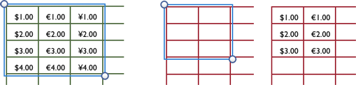
• If you select a group of cells to paste into (rather than a single cell to define the upper-left corner for the paste), and the selection is smaller than what’s on the Clipboard, Numbers pastes only as much as “maps” to the selected target (Figure 49).

Figure 49: Left: A selected (and then copied) block of cells. Right: A selection in the target table and the paste result.

• A paste includes cell formats (border, background, and text attributes), data formats (such as dollar signs and number of decimal places), and comments. You can override this with the Paste and Match Style command, described a few pages ahead in Special Copy and Paste Options.
• When pasting between tables, only “manually” applied cell formats—not those in a table’s style—paste in the new location.
• If you copy a cell range that includes hidden cells—whether you’ve used a Hide command or you’ve filtered that data—the hidden data is pasted only if the targeted paste area matches the copied area in regard to how many hidden cells there are, and where they are. Even if you paste in a spot where Numbers would normally add the necessary rows or columns to accommodate data, the hidden data won’t be pasted unless the hidden rows/columns match.

From (or to) Another App

While it’s fairly straightforward to transfer information from a table in another app to a table in Numbers, you can also paste in text that started in columnar form, with tabs typed between the snippets of information (aka tab-delimited text). (For the purposes of this topic, “table” also means Excel’s window-filling grid.)

Although the following copy-and-paste procedures refer to data coming into Numbers, they generally work in reverse too. Paste a copied swath of cells from a Numbers table into an amicable app, for instance, and you get, depending on the receiving program: the data entered into cells in a spreadsheet or table; a freestanding table made from the copied data; or text separated by tabs and paragraphs.

Note: This topic is all about transferring data by copying and pasting. To learn about exchanging data files, read Importing, Exporting, and Sharing Files.

From a Table

Tables know how to talk to each other when it comes to where pasted information winds up in a Numbers, but when it comes to what—the cell contents—they don’t always speak the same language. And as for cell formats… well, only one other program is fluent in Numbers’ formatting.

Pasting data copied from a table in any of these programs behaves the same as intra-Numbers pastes when it comes to using the correct matrix of cells—even adding rows and columns when necessary—but other paste scenarios have varying mileage:

• Apple’s Pages: Since Pages’ table capability is essentially a clone of Numbers writ small, it’s no surprise that pasted table information comes in completely intact, including any formulas that were copied. If you forget to copy cells referenced by a copied formula, you’ll get an error—but that’s the case with a copy/paste within Numbers, too.
• Microsoft Excel: Static cell contents paste into Numbers without a problem, but formulas don’t survive: Numbers uses only the result of a copied formula (so if you copy a cell containing the formula 2+2, you paste only 4).

  Most data formats (for instance, the number of decimal places, or dollar signs) come through, but it’s as if you had typed them into the cell—the cell doesn’t recognize it as data formatting, and you won’t see it acknowledged in the Format Inspector (see Standard Data Formats). For cell formats, border colors come through, but their pattern and stroke do not; basic text formats are preserved. Cell background fill is erratic, and, when there is color, it doesn’t “register” in the Cell pane as the color fill. In all, remove cell colors and similar formatting before you copy data from Excel.

• Microsoft Word: Paste results are the same as with Excel: flawless in regard to cell contents, unpredictable for cell styles, problematic for data formats, and with formulas translated to their results.

From Text

Inter-app copy/paste operations follow a simple, standard rule: columns are separated by tabs, and rows are delineated by return/paragraph characters. So, if you copy data that’s separated by tabs and divided into lines (which are actually short paragraphs) from any source, it neatly pastes into a Numbers table.

Insert Copied Rows and Columns

Numbers doesn’t make it easy to move rows or columns with the Cut and Paste commands. The problem is that you can’t actually cut a row or column: select it, choose Edit > Cut, and the cell contents are cut, leaving an empty row or column behind, which you must then explicitly delete. How elegant!

Note: For the rest of this section, I’m going to refer to only rows, but everything applies to columns, too. I’ll also focus on single-row operations, but you can do the same with multiple rows.

The best way to move a row or column a short distance is to drag it to the new position (see Move Rows and Columns), because the gap left behind automatically closes.

However, when you’re moving a row beyond the displayed area of a table, dragging can be a problem because it’s easy to overshoot your mark. Instead, try this copy-delete-insert procedure:

1. Select the row (or rows) you want to “move,” and choose Edit > Copy.
2. With the row(s) still selected, choose Table > Delete Row(s).
3. Select the row that’s after the desired insertion spot, and choose Insert > Copied Rows.

Numbers inserts the copied row(s) above the selected row.

You can also use Insert > Copied Rows to move copied rows from one table to another. If you do this and the target table has a different number of columns, the outcome is fairly predictable. If you’ve copied a row shorter than the target table’s, a full row is still inserted. If the target table has shorter rows, new columns are added to accommodate the incoming information; this is not necessarily a Bad Thing, but you should keep an eye on what’s happening to the rest of your table setup.

Using Insert Commands with Text Data

You can paste tab-delimited text into a table and the tabs separate the data into cells, even adding cells to the table if necessary to accommodate the data. Things aren’t as smooth if you use the Insert Copied Row/Column command with text data on the Clipboard:

• Non-Numbers data on the Clipboard overwrites the contents of the current row. It doesn’t insert a new row.
• If you have too many items on the Clipboard (but correctly formatted, with tabs between them), an Insert command truncates the information, chopping off whatever doesn’t fit into existing cells.
• This is a weird one: If you have too few items of information, they will be repeated as many times as necessary to fill the entire row.

Special Copy and Paste Options

So you want to paste data but not the cell and data styles that come along with it. Or maybe you’d like to paste just the formatting information that you painstakingly developed in another table. Or how about pasting just the formula results? Here’s how to do each:

• Paste without formatting: You’ve copied a block of data from another table and want to paste it in your current table without the original cell and data formatting, preferring that it match your current table’s design. Choose Edit > Paste and Match Style (the style being that of the paste location). This also works, of course, for copy/pastes within a table.
• Copy and paste formatting only: Sometimes you want to use that bold, italic, underlined, reddish Hobo text in more than one place, but it’s not worth creating a text style (described in Paragraph and Character Styles). Besides, you want to bring along that yellow-to-black gradient background with the orange dotted border, and the 17-decimal-place custom number format, none of which are included in a text style. The solution isn’t obvious, since it’s not in the Edit menu. But you can copy all the formatting in a selected cell by choosing Format > Copy Style and slap it over other selected cells with Format > Paste Style. This applies to both cell formats (including their text formats) and data formats (which are applied to only “eligible” data in the pasted area—number formats, for instance, are ignored by text-filled cells).

  Since this pastes only the formatting, you can use Paste Style on a cell that has data, and its data remains even if the cell you copied had data in it, too.

• Paste formula results: When you copy cells that have formulas in them, it may feel like you’re copying the result of the formula because that’s what you see in the cell. However, you’re actually copying the formula, and that’s what will be pasted. When you want just the formula result, choose Edit > Paste Formula Results.

  I used Paste Formula Results a gazillion times while creating the examples for this book. I used the RANDBETWEEN function to fill cells with numbers, but since formulas are sometimes automatically recalculated, those numbers would change from one screenshot to the next. So, I copied those cells and then pasted right over them with Paste Formula Results to set the numbers in cement.

Special Data-input Formats

Numbers has five special cell-formatting options that can limit the scope of what data can be entered (only numbers from 1 to 10, for instance), as well as speed up data entry. As a bonus, some of these formats provide at-a-glance information; you don’t have to read a number, for example, when you see a string of stars. The formats are:

• Checkboxes: These simple on/off boxes, covered next, work well in many situations.
• Star Ratings: Clickable stars can represent numbers from 0–5.
• Pop-up Menus: Roll-your-own pop-ups can be populated with any entries you want.
• Sliders and Steppers: These allow input of a defined range of numbers, with or without specific increments.

Checkboxes

Checkboxes are easy to add to a table, and incredibly handy when all you need is to indicate whether a certain condition has been met or not: registered, passed exam, met quota, was present. They let you quickly enter information, and make it easy to scan a column for checked or unchecked boxes.

Note: You can try some checkbox setups in the Numbers templates Attendance (under Education) and Recipe (under Personal).

Set Up Checkboxes

You’d typically add checkboxes to a column that has a header or subheader label describing what the checkboxes stand for—such as the conditions I just mentioned: registered and passed exam.

To set up the checkbox format:

1. Select the cells. (You can select blank or filled cells; Change Data to Checkboxes, a little ahead, describes what happens if the cells contain data).
2. Go to the Format Inspector’s Cell pane.
3. Choose Checkbox from the Data Format pop-up menu.

Numbers puts checkboxes in all the cells. To use the checkbox… well, you know what to do.

Tip: Want to check or uncheck a box without your hands leaving the keyboard? When the cell is selected, type 1 or T (for True) to check the box, and 0 or F (for False) to uncheck it.

Manipulate Checkbox Data

What information does Numbers actually enter when you check or uncheck a box? An unchecked box puts the value FALSE in the cell, while a checked one evaluates to TRUE, as you can see if you look at the Quick Calc bar when a checkbox cell is selected. These are very important values, since they’re used as the basis for IF-statement decisions (described in IF Statements).

To remove a cell’s checkbox formatting, select it and then choose a different format from the Data Format pop-up menu in the Format Inspector’s Cell pane. If you choose Text, you’ll see TRUE and FALSE entries in the cells; choosing Number instead gives you ones (for TRUE) and zeros (for FALSE). As explained in What Is Truth?, these are equivalent values: zeros are false, and non-zero numbers are true.

Change Data to Checkboxes

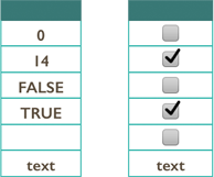
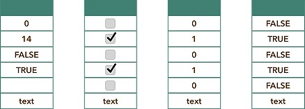
Numbers can translate your data into checkboxes by following simple rules regarding what a checkbox represents: a zero is unchecked, or false, and any non-zero number (including negative values) is checked, or true. Blank cells are unchecked, the words true and false are predictably translated, and any other text is unaffected (Figure 50). Just select the cells and apply checkbox formatting from the Cell pane.

Figure 50: Left: The original data. Right: The data with checkbox formatting applied (including the bottom cell).

Note: You don’t have to input TRUE or FALSE in uppercase for this transition to checkboxes; in fact, you can’t enter them in lowercase, either. The words are so special that if you type either in lowercase, it’s automatically changed to capitals.

Change Checkboxes to Data

To translate checkboxes back to “raw” data, select the cells and choose either Number or Text from the Data Format pop-up menu in the Format Inspector’s Cell pane—but don’t expect your original data to be there: you get only ones and zeros in cells formatted for numbers, and TRUE and FALSE for text cells (Figure 51).

Figure 51: Left to right: The original data; checkbox formatting applied; checkboxes reformatted as numbers; checkboxes reformatted as text. Note that an empty cell is an unchecked box, which turns to a zero when the checkbox formatting is removed.

Represent Data with Checkboxes

You can’t always just change a column of data to checkboxes because it’s easier to read; as you’ve just seen, that can change the underlying data in a way that means you can’t recover it. (In the previous figure, for instance, a 14 is changed to a checkbox, and then changed to either a 1 or TRUE.) But you can create a checkbox column that represents data kept safely elsewhere in the table. This two-step procedure first calculates something from the data, and then turns it into checkboxes, leaving the original data unchanged.

Try it: Use the 5·Budget Checks sheet of The Hands-on Example Spreadsheet.

Make it: Start with Numbers’ Personal Budget template (it’s in the Personal Finance category); add a column (column E), and label it Dif >= $100.

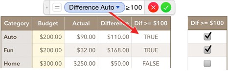
Although we haven’t worked with formulas yet in this book (that’s in Fun with Formulas and Functions), this example is quite straightforward, as you can see in Figure 52 and shouldn’t present a problem whether you’re just reading, or trying it:

1. Type a formula in E2, the first cell in the Dif >= $100 column:
   1. Type the equals sign to open the formula editor.
   2. Click in D2 to enter it in the editor. (The token says Difference Auto rather than D2 because it’s using the labels of the column and row instead of the cell’s column and row coordinates.)
   3. Type >=100 so that the formula is Difference Auto >= 100, and click Accept to close the editor (the >= characters will change to the single ≥). This may not “feel” like a formula, but it is: it’s comparing two values. You see TRUE in the cell, because the value in D2 (Difference Auto) is over 100. (There’s more about TRUE and FALSE values in What Is Truth?.)
2. Autofill from E2 down to the bottom of the table (select the cell, hover near the midpoint at the bottom of the selection, and drag the yellow autofill handle).
3. With the values in column E still selected, go to the Format Inspector’s Cell pane and choose Checkbox from the Data Format pop-up menu.

Numbers changes all the TRUE and FALSE entries to checked and unchecked boxes (Figure 52).

Figure 52: The formula calculates which items are more than $100 over budget; the TRUE/FALSE results can be turned into checkboxes.

Note that this is a one-time, static translation. If you change the values in the table, they won’t be reflected in the checkbox column; the formula you entered was replaced by the TRUE or FALSE result when you changed the cells to checkboxes. If you add rows to the table, you can’t autofill down the checkboxes—you’ll just be copying the last checked or unchecked box.

If you do translate data to checkboxes like this, and think you might have to re-do it later for updated or added data, preserve the formula before you format the cells for checkboxes:

1. Double-click in the first cell where you’ve put the formula to open the formula editor.
2. Press Command-A to select all of the formula; this will ignore the token with the equals sign in it.
3. Press Command-C to copy the formula.
4. Press Return to close the formula editor.
5. Click an empty spot on the sheet to deselect the table.
6. Press Command-V to paste the formula in a text box (you don’t have to insert a text box first—Numbers creates one to accommodate pasted text when nothing’s selected).

Tuck the text box somewhere on your sheet. Should you ever want to reinstate the formula, you can paste the text into the formula editor.

Use Checkbox Data in Formulas

The data stored by a checkbox is a “logical value” of true or false—a concept discussed in IF Statements and Logical Operators. Sometimes, such as when you want to filter rows for those values, you treat them as text, but most of the time you should let Numbers treat them as the special values they are. You’ll see, for instance, in this next example, that true and false values are represented by tokens in a formula.

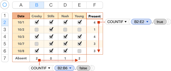
If you want a total for a group of checked or unchecked checkboxes, you can do that with the COUNTIF function, which counts the cells in a range that meet certain criteria. In Figure 53, for example, you can see that the formulas in the Present column give the number of cells in a row that are checked by looking for true values, while the formulas in the Absent row add up the checkmarks in columns by counting the false values.

Figure 53: Count the number of true values in a row to get how many students were present each day; count the false values in a column to total the absences for each student. (The formulas in the cells each refer to their own rows or columns.)

Try it: Use the 6·Attendance Checks tab in The Hands-on Example Spreadsheet.

Make it: Start with Numbers’ Attendance template (in the Education category). Delete all but five body rows by Option-dragging the Row handle upward. The Total footer row won’t be deleted; when it becomes row 7, stop dragging. Delete columns G through I by Option-dragging the Column handle leftward. Erase the data in the footer row: drag across B7:F7 and press Delete. Re-label column F: click in F1 and type Present. Delete the column F data: drag across F2:F6 and press Delete.

We haven’t fully described formulas yet (that’s in Fun with Formulas and Functions), but don’t worry, because the ones in these examples are simple to enter.

To count checked or unchecked boxes:

• Count the checked boxes: See how many students were present each day. Click in F2, type an equals sign to open the formula editor, and enter the formula COUNTIF(B2:E2,true). (Tokens will be offered as you type; ignore them and keep typing.) Close the formula editor with a click of the Accept button. Autofill the formula down through B6.
• Count the unchecked boxes: Check the number of absences for each student. Open the formula editor for B7 by typing an equals sign in the cell, type COUNTIF(B2:B6,false), and click the Accept button. Autofill the formula across through E7.

Star Ratings

When you need to enter only a limited range of values, clicking is quicker than typing. Star ratings let you represent the numbers zero through five by clicking a dot in a cell that turns it, and the preceding dots, into stars.

Warning! You can apply the Star Rating format to cells with existing data, but be careful: anything over 5 is represented by 5 stars, and fractional values are rounded (so 3.4 is 3 stars and 3.5 is 4 stars). If you change the cells back to numeric format, the data remains altered, so the original values are lost.

Star ratings are easy to set up and use:

• Format cells for star ratings: Select the cells and, in the Format Inspector’s Cell pane, choose Star Rating from the Data Format pop-up menu.
• Enter a star rating by clicking: Click a dot to change it to a star, or a star to make it a dot. You don’t have to click the interim dots or stars: to go from 2 stars to 5, just click the fifth star.

  Setting a star rating to zero—no stars—isn’t all that easy (or obvious). Click in the extreme left edge of the cell to turn off all the stars; it’s difficult to avoid hitting the first dot and getting a star.

• Enter a star rating by typing: Select the cell, and then press a number from 0 to 5.

  Be careful when clicking in a star-rating cell, because it’s easy to click a star instead: click in the cell’s extreme corner—the most corner-ish spot you can manage. If a nearby cell is selected, it’s easier to press Tab, Return, or an arrow key to move to the star-rating cell.

• Format the stars:
  • The color of the stars is the text color for the cell. Set it in the Format Inspector’s Text pane, in the Style tab.
  • When you alter a cell’s width, the stars’ spacing, and sometimes size, changes. The stars spread out to fill a wide cell, and if you make the cells taller, the stars get bigger. As a cell gets smaller, the stars also shrink, so that they all remain displayed.
• Use star ratings in formulas: Treat star ratings as numbers in formulas. For example, the table in Figure 54 uses a simple SUM function in the Total column to add the contestants’ points.

Figure 54: Left: In this star-rating table, the final column sums the ratings, which are stored simply as numbers. Right: You can make color-coded star ratings that change color based on the number of stars by using conditional highlighting.

Try it: Enjoy experimenting with star-rating basics in the 7·Chef Stars sheet of The Hands-on Example Spreadsheet. In addition, you can learn how to do the two clever uses of conditional highlighting shown in the figure above: highlighting the highest number in the Total column (in 7·Chef Stars) and setting up the color-change stars (on the 8·Color-Star Ratings sheet).

Pop-up Menus

Numbers’ Autocomplete feature makes it easy to enter data that already exists anywhere in a column. But with the Pop-up Menu cell format, you can create a list of up to 250 entries that needn’t already be in the column—and you can do the same for rows, making repetitive horizontal data entry easier. And because then the only way to enter data is choosing from the menu, input is restricted to those items, not only saving time but also decreasing input errors.

Because Pop-up Menu is a cell format, the menu’s existence depends upon its being in a cell; it can’t exist on its own. If you delete all the cells that use a specific menu, you’ll have to create it all over again.

Note: Throughout this section I describe pop-up menus using column information, but not only can you do the same thing in rows, you can select a block of cells spanning columns and rows to create menus.

Because you’ll be using existing data to create menus, let’s take a quick look at how table data translates into menu items:

• Items in the menu will be in the order in which they appear in the selected cells.
• Blank cells are ignored.
• Repeated entries are ignored, but only if they are exact duplicates: squirrel and Squirrel are not because of the capitalization. On the other hand, 2% and .02 are the same because the underlying numbers are the same (formatting doesn’t count—it’s the data that’s being compared).
• Checkboxes in a selection show in the menu list as TRUE (if they’re checked) or FALSE.
• Star ratings become numbers from zero to five.

Build a Menu

It’s easy to build a menu when you already have data in some cells that are representative of all the items that you want in your pop-up menu. (If your table has only a small proportion of the items you need in your menu, start with Build a Longer Menu, just ahead; it describes how to add temporary menu data to the table.)

Try it: Use the 9·Quick Pop-up sheet in The Hands-on Example Spreadsheet.

Make it: Start with a blank table and enter a short list of food allergies as shown in the next figure (or, really, any text data).

To create a pop-up menu:

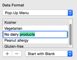
1. Select the cells that contain the information you want in your pop-up menu and the cells where you want the menu to be available (Figure 55), since this procedure both gathers the existing entries and formats the cells for the menus.

   

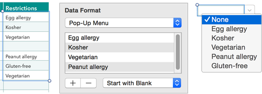
   Figure 55: Left: The selected data. Center: The menu entries in the Cell pane. Right: The pop-up menu for a formatted cell.

   Tip: If you sort the data in the column before you make the menu, your entries—and menu list—will be alphabetical.

2. Go to the Format Inspector’s Cell pane and choose Pop-up Menu from the Data Format pop-up menu.

   Items in the selected cells appear in the menu list.

3. Set a starting item (or not). Choose an option from the menu beneath the item list:
   • Start with First Item: With this very restrictive option applied to a cell, once you open that cell’s menu, you can’t leave the cell without a menu item being entered; if you don’t choose something, the first item is entered as you leave the cell. In addition, when you initially format a cell with this option, the first item in the list is automatically placed in the cell. This is a useful when you want a default cell entry, or if you want to put a prompt in a cell by making something like CHOOSE FROM MENU the first menu choice. Otherwise, it’s incredibly annoying, and makes it very easy to mistakenly populate a table with the wrong data.
   • Start with Blank: This is the better choice in most situations. Cells formatted with this kind of menu start out blank, and if you’ve selected something from the menu and want to delete it, the menu provides a None choice that blanks the cell.

That’s it: click in, or move to, any cell you just formatted, and you see the pop-up menu arrow appear, with a None choice at the top of the menu that was triggered by the Start with Blank option.

Try it: To compare starting with the first item versus a blank, look in the 10·First Item Options sheet of The Hands-on Example Spreadsheet. (It also shows how to use conditional highlighting to show which blank cells are formatted with pop-up menus.)

Build a Longer Menu

Adding more than a few items to a menu list from within the Format Inspector, as I describe just ahead, is tedious at best, but you’ll usually want a full menu before you start your data entry. Here’s how to add temporary data to a column from which you can create a menu list:

1. Add temporary rows to the table, and in the appropriate column, enter the additional items you want in your menu. Since there will be no entries in the other cells of these rows, they will be easy to identify and delete after you create the menu list.
2. Sort the table by the column of data that will make your menu list (see Sorting Data), so that the menu will be in alphabetical order.
3. If you want your menu list mostly alphabetical, with a few specially placed terms, reorder those rows by dragging them into position; this is much easier than moving the items in the menu list later.
4. Create the pop-up menu as just described in Build a Menu, above.
5. Delete the rows you added in Step 1; their entries will remain in the menu list. If the rows are dispersed throughout the table, sort by another column (your fake-data rows are blank everywhere except for the menu-data column) to make it easy to delete them as a group.

Try it: You can try this procedure on the 11·Longer Pop-up sheet in The Hands-on Example Spreadsheet.

Edit a Menu List

No matter how carefully you plan, you’ll probably need to edit your menu list eventually: add a new item, get rid of an existing one, reorder the list, correct a misspelling, and so on.

When you edit a menu list, start by selecting the cells that are formatted for the menu. You can’t see the menu list in the Format Inspector unless at least one cell with the menu in it is selected, but if you don’t select them all, you’ll end up with some cells using the old version of the menu, and some using the new. (Combine Menu Lists can help you with that situation.)

With your cells selected, work in the Format Inspector’s Cell pane to:

• Edit an existing item: Double-click an item in the list to activate it, edit it (Figure 56), and then press Return to deselect the item. This changes not only the menu, but also any cell that contains the original entry as long as the cell is selected when you make the change to the list.

Figure 56: Select an item to edit it.

Note: You can click anywhere in an entry to select an item. To select text for editing, however, you must click on the text. A single click works if the line is already selected; otherwise, double-click the text.

• Add an item: Click the Add button beneath the list and type the new entry in the framed line in the list. A new entry is always added to the bottom of the list, no matter which line is selected when you click the button. (If you didn’t start your menu list with an existing column of data, this is how you’d build the entire menu list.)
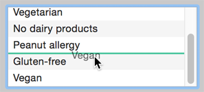
• Reorder the list: Simply drag items in the menu list to their new positions (Figure 57).

Figure 57: Drag to reorder items in the menu list.

• Remove an item: This is particularly useful (not to mention needed) if you’ve selected a whole column and turned it into a menu list, mistakenly including a header cell. Working in the Format Inspector, with the to-be-formatted cells selected, select an item and click the Remove button beneath the list.

  Cells that had been filled with the removed item (and are part of the current selection) revert to the starting item you specified: a blank or the first item in the list.

Combine Menu Lists

If you set up a column with pop-up menus, and then carelessly edit a menu list without selecting all the cells first—and maybe even do it more than once so that you have several different menus in the column—you don’t have to start again:

1. Select all the cells in the column that you want to standardize to a single menu.
2. In the Format Inspector’s Cell pane, click the Merge Menu Items button that appears in the Data Format section beneath the menu where you selected Pop-up Menu. (If there’s no Merge Menu Items button, then all the selected cells already have the same menu.)

You’ll probably want to fine-tune the combined list. Numbers filters out duplicates, but things you deleted from one version of the menu will reappear in the combined version, or you may have what are essentially duplicates (“Egg allergy” and “Egg allergies”). You also may need to reorder the list.

Work with Pop-up Menu Cells

When you go to a cell with a pop-up menu, a tab with a menu arrow in it appears to the right of the cell; click it to pop open the menu, and choose an item. You can also:

• Access the menu from the keyboard: When the cell is selected, press the Space bar to open the menu, navigate it with arrow keys or by typing a few letters to identify your choice, and close it with a press of Return, Space bar, or Esc.
• Remove the menu but leave the data: Select the cell(s), open the Format Inspector’s Cell pane, and choose Automatic or Text from the Data Format pop-up menu.
• Restore a menu deleted by mistake: If you delete the contents of a cell, its formatting—in this case, the menu—disappears, too, and you might not realize it until it’s too late to undo. To reapply the formatting to an empty cell: select a cell that still has the menu, choose Format > Copy Style, go back to the emptied cell, and choose Format > Paste Style. This pastes the menu in the new spot, but ignores the data from the copied cell.

Sliders and Steppers

When you have cells that are for only numeric input—and, more specifically, numbers in a predetermined range with perhaps even definable internal increments—you don’t have to create pop-up menus to keep data entry accurate. Instead, you can format the cells for a slider or a stepper input control.

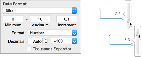
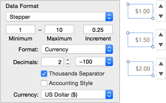
A slider-formatted cell pops up a vertical bar; slide the ball up or down to change the number in the cell. A stepper control provides up and down arrows, which you click to increment or decrement a number. I recommend the former for all but a very narrow range of numbers, as clicking the arrows on a stepper input is incredibly tedious.

To set up a slider or stepper:

1. Select the cells to be formatted, and go to the Format Inspector’s Cell pane.
2. In the Data Format section, choose Slider or Stepper from the pop-up menu. (Use sliders when there are more possibilities to be accommodated: a smaller increment, a larger range, or both.)
3. Enter minimum and maximum values and any increment you need.
4. Configure your slider or stepper further with the Format pop-up menu and the controls beneath it (Figure 58 and Figure 59).

Figure 58: Left: The setup for a slider control. Right: Sliders pop out from formatted cells.

Figure 59: Left: The options for the Stepper control. Right: The results of repeated clicks in the control for a formatted cell; the values increment by .25, as defined.

Numbers applies your stepper or slider to the selected cells.

Try it: Experiment with these controls in the 12·Steppers & Sliders sheet in The Hands-on Example Spreadsheet.

Here’s what you need to know about using sliders and steppers:

• Enter a value: Click in a cell to see the slider or stepper, and pick a value. You can also ignore the controls and just type a number into the cell.
• Out-of-range-values: If you type a number outside the defined range, it changes to the lowest or highest allowable entry.
• Non-incremental values: If your entry doesn’t match a defined increment, it’s rounded to the nearest one. Entering 10.2 when the cell is formatted for increments of .5 rounds to 10.0.
• Remove the slider/stepper but keep the data: Select the cell(s) and, in the Format Inspector’s Cell pane, choose Number from the Data Format pop-up menu.

Tip: You don’t have to keep clicking the stepper arrow: “press” it by keeping your mouse button or trackpad down, and the number increments or decrements. Nor must you always slide the slider ball; click anywhere on the bar and the ball jumps to that position.