1

Getting Started

In this chapter we will take a brief tour of Mathematica, a program for modern technical computing based on the Wolfram Language. It is important to read this chapter carefully since its contents are essential to be able to follow the rest of the book. Even if you are already a Mathematica user, you may find the following pages useful to get familiar with the new functionality included in the most recent program releases.

1.1 Mathematica, an Integrated Technical Computing System

Mathematica is a software application that goes beyond numeric and symbolic calculations. It is a modern technical computing system based on a high-level general-purpose programming language, the Wolfram Language. You will be able to start using it after a few minutes but, if you want to take full advantage of its capabilities, you will have to spend time to master its language although probably less than with other programming languages.

Mathematica took a revolutionary step forward in Version 8 with the introduction of the free-form linguistic input, that consists of writing in plain English a request that the program will try to answer. Using this format ensures that newcomers can get started very quickly. For experienced users, it means help in finding the most appropriate functions to perform a desired calculation. To get an idea of Mathematica’s capabilities before beginning to use the program, let’s take a look at the following examples (for now, you just need to read what follows, later we will show you how to write inputs and run commands):

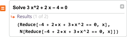
• To solve an equation such as 3x² + 2x − 4 = 0, you can literally type what you want Mathematica to do. The output shows the correct Mathematica input syntax and the answer, which in this case includes both, the exact solution and the decimal approximation.

  

  {x=13(−1−13)∨x=13(13−1),x=−1.53518∨x=0.868517}

• To add quantities in different currencies, just enter them and the result is shown in the currency that was used first; if you execute the command, the result will most likely be different due to changes in the exchange rates from the time the input was first executed.

  

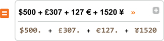
  $1061.78

• We can even ask very specific questions: To learn more about the temperature in a location, just write down the name of the place followed by “temperature”. The most important advantage is that the information from the answer can be used inside the Mathematica environment.

  

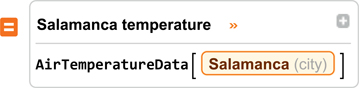
  17.3°C

The Mathematica free-form input is integrated with Wolfram|Alpha, http://www.wolframalpha.com, a type of search engine that defines itself as a computational knowledge engine and that instead of returning links like Google or Bing, provides an answer to a given question in English. If you want, you can access Wolfram|Alpha directly from within Mathematica, and we will show you how to do that later on.

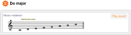
• To represent the Do major music scale, you just need to write:

  

Another example of the new functionality recently incorporated in Mathematica is the possibility of accessing scientific and technical databases through the Internet from different fields already formatted by Wolfram Research for their direct manipulation inside the application.

• In this example, we obtain the value of the Euro in US dollars after executing the command.

     FinancialData ["EUR /USD"]
  
     1.0661

• We can choose a chemical compound and get many of its properties. In this case, we get the plot of the caffeine molecule.

     ChemicalData ["Caffeine", "MoleculePlot"]

  

With very brief syntax we can build functions that in other programming languages would require several lines of code.

• With just two lines of commands we can generate a dynamic clock that is synchronized with the time in our computer and in a different time zone.

  Dynamic [Refresh [Row[
     {ClockGauge[AbsoluteTime[], PlotLabel -> Style["Local", Large, Bold]],
      ClockGauge[AbsoluteTime[TimeZone] → +9],
       PlotLabel -> Style["Tokyo", Large, Bold]]}], (UpdateInterval -> 1)]]

  

• In less than half a line we can write the necessary instructions to make an interactive model of the Julia fractal set.

    Manipulate[JuliaSetPlot [0.365 - k İ,
      PlotLegends → Automatic, ImageSize → Small], {k, 0.4, 0.5}]

  

• We find the intersection points of a circumference and a parabola and graphically represent them. To write special symbols such as “∧”, the best thing to do is to use Palettes, which we will discuss later on.

  pts = Slove[x2+y2=1∧y−2x2+32=0,{x,y}]{{x→−1212(5−5),y→14(−1−5)},{x→1212(5−5),y→14(−1−5)},  {x→−1212(5+5),y→14(5−1)},{x→1212(5+5),y→14(5−1)}}

     Show[
      {ContourPlot[{x2+y2=1,y−2x2+32=0}, {x, -1.5, 1.5}, {y, -1.5, 1.5}],
       Graphics[{Red, PointSize[Medium], Point[{x, y} /. pts]}]}]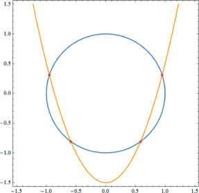

  

Apart from the examples given above showcasing some of Mathematica’s new functionality, it is also worth mentioning: (i) The Wolfram Predictive Interface, that makes suggestions about how to proceed after executing a command, (ii) The context-sensitive input assistant to help us choose the correct function, (iii) The possibility of running the program from the browser (WolframCloud.com), including specific cloud-computing related commands, (iv) The machine learning capabilities that, for example, enable us to analyze a handwritten text and keep on improving its translation through repetition, (v) Very powerful functions for graphics and image processing. We will refer to these and other new capabilities later on.

1.2 First Steps

The program can be run locally or in the cloud accessing the Wolfram Cloud (http://www.wolframcloud.com/) with a browser. From here on, except mentioned otherwise, it will be assumed that you have installed Mathematica locally and activated its license. When installing it, an assistant will guide you through the activation process. If this is the first time, it will take you to the user portal (https://user.wolfram.com), where you will have to sign up. The website will ask you to create a Wolfram ID, use your email address, and your own password. It will also automatically generate an activation key. Remember your Wolfram ID and password because they will be useful later on if, for example, you would like to install the program in a different computer or have an expired license. In both cases, you will need a new activation key. The Wolfram ID and password will also be necessary to access the Wolfram Cloud, and we will give a specific example at the end of the chapter.

To start the program in Windows, under the programs menu in your system, click on the Mathematica icon. Normally there are two icons; choose Mathematica and not Mathematica Kernel.

Under OS X, the program is located in the applications folder and you can launch it either locating it with Finder, using the Dock or from the launchpad (OS X Lion or more recent versions).

By default, a welcome screen (Figure 1.1) similar to this one will appear:

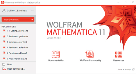
Figure 1.1     The Welcome Screen in Mathematica 11.

This screen contains several external links (hyperlinks). For example, by clicking on Resources, you will be able to access a broad collection of reference materials about how to use Mathematica, including videos: http://www.wolfram.com/broadcast/. You can always go back to this screen from the menu bar: Help ▶ Welcome Screen... . In the upper left-hand corner (in Mathematica 10/11) you will see this icon: . If you are a registered user, chances are you already have a Wolfram ID. In that case, click on the icon and sign in. Once the process has been completed, the icon will be replaced with the name that you used when you signed up, as shown in the previous image. The advantage of this is to gain access from within Mathematica to your files in the cloud (WolframCloud) but for now, you can skip this step if desired. If you click on NewDocument, below the icon shown at the beginning of the paragraph, a new blank Notebook will be created. Notebooks are the fundamental way to interact with Mathematica. You can also create them by clicking on File ▶ New ▶ Notebook.nb.

A notebook is initially a blank page. We can write on it the text and instructions that we want. It is always a good idea to save the file before we start working on it and, as in most programs, this can be done in the menu bar: File ▶ Save As ▶ “Name of the File” (Mathematica by default will assign it the extension .nb).

It is always convenient to have access to the toolbar from the beginning of the session; to do that, select in the menu bar Window and check Toolbar ▶ Formatting (or Show Toolbar in Version 9 and earlier). Please note the drop-down box to the left of the toolbar (Figure 1.2), that we’ll refer to as: style box. It will be useful later on.

Figure 1.2     Mathematica’s Formatting Toolbar.

Once you begin to type, a new cell will be created. It will be identified by a blue right-bracket square (]) (“cell marker”) that appears on the right side of the notebook. Each cell constitutes a unit with its own properties (format, evaluable cell, etc.). To see the cell type, place the cursor inside or on the cell marker. The type will appear in the style box (Figure, Input, Text, Title, Program...). We can also change the format directly inside the box. Type in a text cell and try to change its style.

This is a cell formatted using the Program style.

When a blank notebook is created, it has a style (cell types, fonts, etc.) that assigns to each type of cell certain properties (evaluable, editable, etc). The first time a notebook is created, Mathematica assigns a style named Default (by default). Later on we will see how to choose different styles. In the Default style, when a new cell is created, it will be of the Input type, which is the one used normally for calculations. When we evaluate an Input type cell, “In[n]:= our calculation” will be shown and a new cell of type Output will be generated where you will see the calculation result in the form of “Out[n]:= result” (n showing the evaluation order). However, in this book we sometimes use an option to omit the symbols “In[n]:=” and “Out[n]:=”. These and other options to customize the program can be accessed through Edit ▶ Preferences ....

To execute an Input cell select the cell (placing the cursor on the cell marker) and press or on the numeric keypad. You can also access the contextual menu by right-clicking with the mouse and selecting “Evaluate Cell”.

2 + 2

4

Figure 1.3     The Suggestions Bar.

Since Mathematica 9, when a cell is executed, a toolbar appears below its output as shown above (Figure 1.3). This bar, named the Suggestions Bar, provides immediate access to possible next steps optimized for your results. For example, If you click on range you will see that a new input is being generated and a new suggestions bar will appear right below the result:

Range [4]

{1, 2, 3, 4}

The Suggestions Bar is part of the predictive interface. It tries to guide you with suggestions to simplify entries and ideas for further calculations. It is one more step to reduce the time it takes to learn how to use the program.

All written instructions inside a cell will be executed sequentially. If at the end of an instruction we type semicolon ";", the instruction will be executed but its output will not be shown. This is useful to hide intermediate results. In an evaluation cell (Input) we can include one or more comments, writing them in the following format: (* comment *). Nevertheless, it is recommended to include the comments in separate cells in text format. Remember that you can do that by choosing Text in the style box.

To create a new cell we just need to place the cursor below the cell where we are and then start writing. We can also create a new cell where the cursor is located by pressing .

To facilitate writing, Mathematica provides Palettes. These can be loaded by clicking on Palettes in the menu bar. There are several palettes to make it easier to type mathematical symbols such as the Basic Math Assistant palette or Other ▶ Basic Math Input. It would be useful from now on to keep one of them open.

Alternatively, you can use keyboard shortcuts to write special symbols, indexes, subindexes, etc. The most useful ones are: subindex , superindex or , fraction and the square root symbol . Depending on your keyboard configuration, to use some of the previous symbols you may have to press first (key CAPS) for example: superindex .

• Using a palette or the keyboard shortcuts write and execute the following expression. Please remember: an empty space is the equivalent of a multiplication symbol: that is, instead of 4×5 you can write 4 5.

  4×55+4−32−3

The previous Input cell was written in the standard format (StandardForm). It is the one used by default in Input cells. To check it, position the cursor on the cell marker and in the menu bar choose: Cell ▶ Convert To ▶. StandardForm will appear with a check mark in front of it.

Expressions can also be written without the need for special symbols by using the form: InputForm. It is very similar to the one used by other programming languages such as C, FORTRAN or BASIC. For instance: multiplication = " * ", division = " / ", addition = " + ", subtraction " = ", exponentiation =" ^ ", and square root of a = "Sqrt [a]". We can replace the multiplication symbol by an empty space. It is very important to keep that in mind since Mathematica interprets differently "a2" and "a  2": "a2" is a unique symbol and "a  2" is a*2.

• In InputForm the previous expression can be written as:

  (4*5)/5 + Sqrt[4] - 3^2

  −3

Initially, it was its symbolic calculation capabilities that made Mathematica popular in the academic world.

• As an example, write and execute the following in the standard form in an input cell (use a palette to help you enter the content).

  ∂x,y Sin [x y]cos(xy)2y−12x sin(xy)

A customized style, to which we will refer later, has been defined in this notebook so that the outputs are shown in a format that corresponds to traditional mathematical notation. In Mathematica it is called TraditionalForm. We could have defined a style so that the inputs also use the traditional notation as well, but in practice it is not recommended. However, you can convert a cell to the TraditionalForm style anytime you want.

• Copy the input cell from above to a new cell and in the menu bar select Cell ▶ Convert To ▶ TraditionalForm. Notice that the cell bracket appears with a small vertical dashed line. You will be able to use the same menu to convert to other formats.

  ∂2 sin(xy)∂ x ∂ ycos(xy)2y−12x sin(xy)

For Windows, since Windows 7, you can use the Math Handwriting Input, available under accessories, to write the entries manually using a tablet or an electronic board.

The linguistic or free-form format (available since Mathematica 8) allows us to write in plain English the operation we want to execute or the problem we want to solve. To start using it press = at the beginning of the cell (input type) and you will notice that will appear. After that write your desired operation. Your instruction will automatically be converted into standard Mathematica notation, and after that the answer will be displayed. Let’s take a look at some examples.

• To add from 1 to 10 you can write “sum 1 to 10” or other similar English expressions such as “sum from 1 to 10”.

  

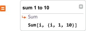
  55

If you follow the previous steps, the entry proposed may be different from the one shown here. The reason behind this is that when using the free-form format, the program connects to Wolfram|Alpha, Wolfram’s computation knowledge engine, that is constantly evolving.

Move the cursor over Sum {i, 1, 10}] and the message “Replace cell with this input” will appear. If you click on the symbol located in the upper right-hand corner, additional information about the executed operation will be shown.

If you have received any message related to connection problems, it is because the free-form format and the use of data collections that we will refer to later on, requires that your computer is connected to the Internet. If it is and you still have connectivity problems it may be related to the firewall configuration in your network. In that case you may have to configure the proxy (see http://support.wolfram.com/kb/12420) and ask for assistance from your network administrator.

When you don’t know the correct function syntax, you can use the free-form format to write what you want to do. Mathematica probably will show you the correct syntax immediately, click on it and only the input in the correct notation will remain with the free-form format entry disappearing.

The free-form input format generally works well when it’s dealing with brief instructions in English. In practice it is very useful when one doesn’t know the specific syntax to perform certain operations in Mathematica.

Many more examples can be found in:

http://www.wolfram.com/mathematica/new-in-8/free-form-linguistic-input/basic-examples.html.

It’s also very useful to use Inline Free-form Input.

• In this example, we assume we don’t know the syntax to define an integral. In an input cell we click on Insert ▶ Inline Free-form Input and will appear. Inside this box we type integrate x^2.

  

  x33

• The entry is automatically converted to the standard syntax in Mathematica.

  

  x33

• By clicking on the above input over the symbol, the cell will go back to its free-form format .

  

  x33

• In the following example we have used Inline Free-form Input writing integrate cos x from 0 to x.

  

  sin(x)

• By clicking in the input is automatically converted to the standard syntax in Mathematica. It can be used as a template.

  Integrate [Cos[x], {x, 0, x}]

  sin(x)

• The command below returns the average acceleration of the gravity g on earth at sea level.

  

  9.80 m/s²

  By default the units used are the ones from the international system (SI):

• Here we combine a standard function inside the Inline Free-form Input with QuantityMagnitude that shows the numeric value, without including the units:

  

  9.80

As we have indicated in the introduction, you can directly access Wolfram|Alpha from Mathematica. To do that just press the equal sign on your keyboard twice (“==”) at the beginning of an input cell. The symbol will appear, then type what you want.

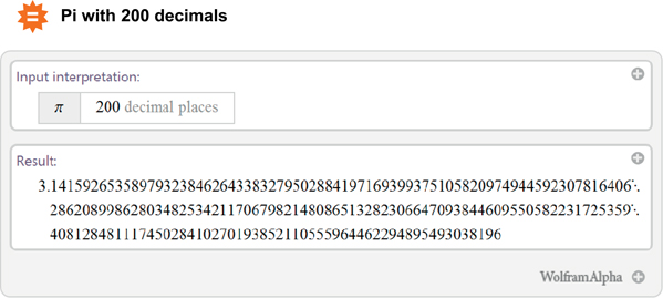
• Let’s go back to one of our introductory examples:

  

  From the output, not shown, we selected the part that we were interested in (“Music notation”) by clicking on the symbol and choosing the desired option (“Formatted pod”). A new entry was generated showing only the musical scale.

   WolframAlpha ["Do major",
    IncludePods → "MusicNotation", AppearanceElements → {"Pods"},
    TimeConstraint → {30, Automatic, Automatic, Automatic}]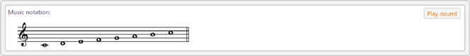

  

  If you click on Play sound you will hear the sound.

The most important difference between using the free-form input notation and the Wolfram|Alpha one, is that in the first case the entry that we write is sent by the program to a Wolfram server that will return the syntax in Mathematica and it will be executed locally, while by using the Wolfram|Alpha notation, all the processing is done in the server and our computer only displays the output. If we have Mathematica it is better to use the free-form notation to get the Mathematica syntax and then we will be able to use the output easily in subsequent calculations.

Wolfram|Alpha is very useful from a browser since we don’t need to have the program installed: There are applications -Apps- for smart phones and tablets that facilitate its use and Widgets developed with it.

Besides all the previously described ways to define the cell type, there is another one that consists of placing the cursor immediately next to the cell to which you want to add another one. You will see “+” below the cell to its left. Click on it and choose the cell type that you want to define: Input, , , Text, etc.

1.3 The Help System

If you have doubts about what function to employ, the best approach in many cases is to use the free-form input format and see the proposed syntax. However, if you would like to deepen your knowledge about the program you will have to use its help system.

The help system consists of different modules or guides (Help ▶ Wolfram Documentation) from where you can access an specific topic with its corresponding instructions (guide/...). Additionally, you will find tutorials and external links. Clicking on any topic will show its contents.

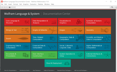
Figure 1.4     The Wolfram Language Documentation Center.

In the screen-shot shown above (Figure 1.4), after clicking on Data Manipulation & Analysis

▶ Importing & Exporting Mathematica displays the window below (Figure 1.5). Notice that besides giving us the functions related to the chosen topic, we can also access tutorials and even external resources such as video presentations.

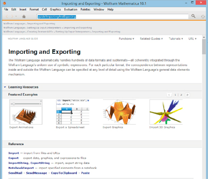
Figure 1.5     How to import and export using Mathematica.

If we don’t have a clear idea of the function we want to use or we remember it vaguely, we can use the search toolbar (Figure 1.6) with two or three words related to what we are looking for.

Figure 1.6     The Search Toolbar.

Another type of help is the one given when a mistake is made. In this case we should pay attention to the text or sound messages that we may receive. For example, if we try to evaluate the following text cell, we will receive a beep.

“This is a text entry”

With Help ▶ Why the Beep?... we will be able to know the reason behind the beep.

Another additional source of help is the Input Assistant with its context-sensitive autocompletion and function templates features: when you start writing a function, Mathematica helps you automatically complete the code (similar to the system used by some mobile phones for writing messages). For example: If you start typing Pl Mathematica will display all the functions that start with those two letters right below them (Figure 1.7). Once you find an appropriate entry, click on it and a template will be added.

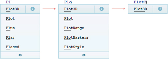
Figure 1.7     The Input Assistant in action.

Sometimes a down arrow will be shown at the end of the function offering us several templates (Figure 1.8). Choose the desired one.

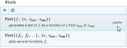
Figure 1.8     Function templates for the Plot function.

Additionally, a color code enables syntax error detection. If you have written a function and it is shown in blue, probably it has not been typed correctly. All Mathematica and user-defined functions will be shown in black. For example: Write in an input cell Nmaximize, it will be shown in blue, write NMaximize and you will see that it is shown in black and a template is displayed.

1.4 Basic Ideas

Users with prior knowledge of other programming languages such as C or FORTRAN, very often try to apply the same style (usually called procedural) in Mathematica. The program itself makes it easy to do so since it has many similar commands such as: For, Do, or Print. Although this programming style works, we should try to avoid it if we want to take full advantage of Mathematica’s capabilities. For that purpose we should use a functional style, that basically consists of building operations in the same way as classical mathematics.

This section is for both the uninitiated into Mathematica and those Mathematica users that still use procedural language routines. Because of that, if you have ever programmed in other languages please try not to use the same programming method.

In this brief summary we will refer to some of the most frequently used commands and ideas. We will usually not explain their syntax or we’ll do it in a very concise way. For additional details, just type the command, select it with the cursor and press <F1>. If you don’t understand everything that you read, don’t worry, you will be given more details in later chapters.

When you don’t know the syntax of a function, type it, select it with the cursor and press the <F1> key.

1.4.1 Some Initial Concepts

• Let’s begin by writing the expression below.

  

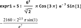
We have assigned it the name expr1, to be able to use the result of the calculations later on. To write the transcendental numbers π and we have used special symbols ( is not the same as e, e is a letter without any other meaning) located in one of the palettes. If we prefer to use the keyboard we can write Pi for π and E^ or Exp[] for . Notice that we use a single equal sign "=" to indicate sameness or equivalence in equations. For comparisons, we will use the double equal sign "==".

• The same operations can be written as in the cell below, using the typical InputForm notation.

  (5! 6^2/2^ (1/3) Pi Cos[3 Pi] Sin[1]) / E^7 (*This is a commment*)

  

  We have included a comment inside the actual cell "(* comment *)". This comment will be neither considered in the computation nor shown in the output.

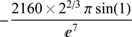
Naturally, in both cases we obtain the same result. There is something that should draw our attention in this output. Apparently, there are terms that have not been evaluated and that appear again as such: π, Sin[1], y ⁷. This is because Mathematica does not simplify or make approximations if that means losing precision. It literally works with infinite precision. Nevertheless, we can force it to compute the decimal approximation, the usual approach in other programs. To do that we will use the function N as shown in the next function. A similar result can be obtained by including decimals in some of the numbers.

• In this example we use the % symbol that recalls the last output. //N or N[expr] will use in the calculations machine precision even though the output may show fewer decimals.

  % //N

  −8.26548

• Another option is to substitute the number with a decimal approximation. You can try in the previous example using Sin[1.0] instead of Sin[1]

• By default 5 decimals are shown, but with N[expr,  n] we can use a precision n as large as desired.

  N[expr1, 30]

  −8.26547962656679448059436738241

Mathematica contains thousands of prebuilt commands or functions (Functions) that are always capitalized. The program differentiates between lower and upper cases. For example: NMinimize is not the same as Nminimize. Arguments are written inside square brackets [arg]. However, users can define a function using lower case.

Lists are a fundamental Mathematica concept, frequently used in many contexts. In a list elements are inside curly brackets {}. Later on we will refer to them.

Remember: All functions in Mathematica are capitalized: Log; arguments are written inside square brackets: Sin[2 x + 1]; list elements are inside curly brackets: {a₁, ..., a_n}; ranges are written as lists: Plot[x, {x, 0, 2 Pi}] ; parentheses are used to group operations: (Log[a x] + Sin[b x])/(a - b).

Use the help to investigate the various functions and their arguments. Remember that you can select a function with the cursor and press <F1> to get information about it. Besides its syntax, examples, tutorials and other related functions are displayed.

• Write Pl in an input cell. The context-sensitive input assistant will show you all the functions that start with Pl. Select Plot. Next to Plot a new down arrow will appear. Click on it and a template like the one shown below will be created.

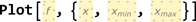
Figure 1.9     Template for the Plot function.

The cell above is an input type cell. If you’d like to avoid its evaluation: Cell ▶ Cell Properties and uncheck Evaluable. That is what we have done in this case in the original document since the idea is to see the cell content but not to execute it.

• In the previous template, all the basic function arguments are displayed. Now you can fill them in using the options as the next example shows. Execute the command.

  

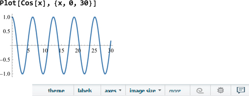
  Figure 1.10     The Suggestions Bar for plots.

• The resulting output is a plot with the suggestion bar (Figure 1.10) appearing right below it.

  Since Version 9, thanks to the WolframPredictiveInterface, the Image Assistant and Drawing Tools provide point-and-click image processing and graphics editing. Click on theme... and a menu with several choices to customize the plot will unfold (Figure 1.11).

  

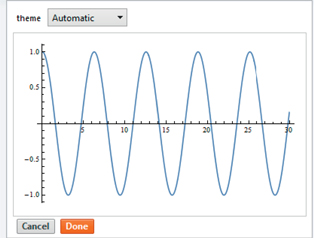
  Figure 1.11     Customizing a plot using the “theme...” option in the Suggestions Bar.

• Alternatively, or if you are using a version prior to 9, you can customize the plot using the Plot options directly (type Plot, select it with the mouse and press <F1> to see them).

Besides arguments, commands also have options. One way of seeing those options directly is Options[func]:

• Solve options:

  Options [Solve]

  {Cubics → True, GeneratedParameters →C, InverseFunctions → Automatic,

  MaxExtraConditions → 0, Method → Automatic, Modulus → 0,

  Quartics → True, VerifySolutions → Automatic, WorkingPrecision → ∞}

Next, we’ll show some examples. Replicate them using the Basic Math Assistant that includes templates for hundreds of commands.

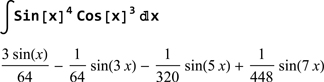
• Definite integral example:

  

• Use Simplify anytime you need to simplify a complex expression.

  Simplify [x⁸ - 4x⁶ y² + 6x⁴ y⁴ - 4x² y⁶ + y⁸]

  (x² - y²)⁴

There are also other commands to manipulate expressions. You can find them in the palette Other ▶ Algebraic Manipulation. Note that you can manipulate an entire expression or just part of it.

• Try to use it with this example simplifying the Sin and Cos arguments separately.

  Sin[x⁸ - 4x⁶ y² + 6x⁴ y⁴ - 4x² y⁶ + y⁸] [Cos[x⁴ + 2x² y² + y⁴]

• To get:

  Sin[((x² - y²)⁴)]/Cos[(x² + y²]²]

• In this example a random distribution of spheres in a three-dimensional space is shown.

  Graphics3D[
   {Yellow, Sphere [RandomInteger [{-5, 5}, {10, 3}]], ImageSize → 250}]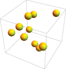

  

You can rotate the image to see it from different angles by clicking with the mouse cursor inside.

If you haven’t used Mathematica previously, the last command may seem strange. Let’s analyze it step by step:

• Highlight RandomInteger and press <F1>. The help page for the command will be displayed. In this case with RandomInteger [{-5, 5}, {10, 3}] we are generating 10 sublists with 3 elements, each element being a random number between -5 and 5. We are going to use them to simulate the coordinates {x, y, z}.

• The previous command is inside Sphere (do the same, highlight Sphere and press <F1>) a command to define a sphere or a collection of spheres with the coordinates [{{x₁, y₁, z₁}, {x₂, y₂, z₂}, …}, r], where r is the radii of the spheres. If omitted, as in this example, it’s assumed that r = 1.

  Sphere[RandomInteger [{-5, 5}, {10, 3}]]

  Sphere[(23041−14−4−3−524−23−2−4−52−1−3315−5−4−2−15−4−1)]

  Note: In this particular notebook, list outputs are sometimes shown as matrices.

We use the command Graphics3D to display the graphs. We have added Yellow to indicate that the graphs, the spheres in this case, should be yellow and the option ImageSize to fix the graph size and make its proportions more adequate for this example. Finally we arrive at the command: Graphics3D[{Yellow, Sphere[RandomInteger[{-5, 5}, {10, 3}]], ImageSize → 250}].

When you don’t understand an instruction consisting of several different commands, decompose it into its individual instructions and analyze each one separately using the help system.

• In the next cell we use Rotate to show a rotated output, in this case by 1 radian, compared to the usual display.

  Rotate[1/Sqrt[1 + x], 1]

  

  Type inside the output and you’ll see that it retains its properties.

• Practically anything can be used as a symbol. Generate a small red sphere.

  Graphics3D [{Red, Sphere[]}, ImageSize → 30]

  

• Substitute the symbol thus obtained, , pasting it below replacing b and evaluating the cell.

  

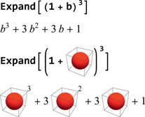
1.4.2 Replacements

A replacement consists of a rule to substitute one or several symbols with other symbols or values. To do that you apply the following syntax: "exp /. rule" that will replace exp with the contents of rule.

• In the expression a x + b y, a is replaced with 3 and b with 5, using a replacement rule.

  exp1 = ax + by / . {a → 3, b → 5};

• From now on anytime we call exp1 we will see that the replacement has taken place:

  exp1

  3 x + 5 y

If you apply several replacement rules to the same expression in succession, the replacement takes places consecutively:

• We first apply the rule (/.a→b) to the expression a x + b y and then the second rule (/.b→c) is applied to the previous result.

  a x + b y / . a → b / . b → c

  c x + c y

• In the expression below we make an assignment that consists of assigning the symbol sol to the solution of a x² + b x + c == 0.

  sol = Solve[a x² + b x + c == 0, x];

• The output is a list.

  sol

  {{x→−b2−4a c−b2 a},{x→b2−4 a c−b2 a}}

  Remember that for assignments a single equal sign "=" is used, while to indicate an equality in an equation or a comparison, we will use a double equal sign "==" that when typed will be automatically converted to “==”.

• To verify that the previous result represents the solutions to the equation ax² + bx + c == 0 we use the replacement "exp /. rule" that will replace in exp whatever is specified in rule.

  a x² + b x + c = 0 /. sol

  {(−b2−4 a c−b)24 a+12 ab(−b2−4 a c−b)+c=0,  (b2−4 a c−b)24 a+12 ab(b2−4 a c−b)+c=0}

We can see that the replacement has taken place, but it’s convenient to simplify it. For that we’ll do as follows: we use Simplify [%] where % enables us to call the result (Out) of the last entry and evaluate the cell.

• We will check that effectively the equality holds and therefore the solution is correct. In this case it was evident, but we can apply the same method to more complex situations.

  Simplify [%]

  {True, True}

When an assignment is not going to be used later on, it may be convenient to delete it using the command Clear.

• The following command removes the assignment previously associated to sol.

  Clear[sol]

• Now, when we type sol we see that it has no assignment.

  sol

  sol

1.4.3 Functions

Mathematica makes it easy to define functions in a way very similar to regular mathematics. The usual syntax in the case of a function of one variable is: f[x_]:= expr[x]. The blank ("_") next to the variable is used to specify the independent function variable.

• Let’s see it with an example.

  f[x_] := 0.2 Cos[0.3 x²]

• Now we can assign a value to the independent variable and we’ll get the function value.

  f[3]

  −0.180814

• We could have also typed the previous two operations in the same cell (don’t forget in this case to enter “;” at the end of each function). However, it’s better to use one cell for each function until you have enough practice. It will help you find mistakes.

  f[x_] := 0.2 Cos[0.3 x²];

  f[3]

  −0.180814

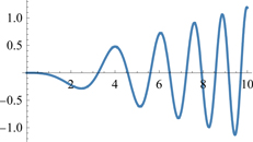
• Now we are ready to visualize the Derivative (') of f[x] in a specific interval.

  Plot[f' [x], {x, 0, 10}]

  

• The same approach can be extended to several variables. In this example we use the previously defined f(x) function.

  g[x_, y_] := f[x] 2.3 Exp[- 0.3 y²]

• Now we can present the result in a 3D graph using Plot3D. We use the option PlotRange -> All to display all the points in the range for which the function is calculated, remove the option to see what happens.

  Plot3D[g[x, y], {x, -2π, 2π}, {y, - 2π, 2π}, PlotRange -> All]

  

1.4.4 Dynamic Assignment of Variables

We can make dynamic assignments in which the symbol (make sure that in the menu bar Evaluation ▶ Dynamic Updating Enable is checked) returns an entry that changes dynamically as we make new assignments to it.

   Clear [a]

• Let’s create a variable.

  Dynamic [a]

  a

• If we now assign to a different values or expressions, you’ll see that the output above keeps on changing.

  a=255a=Integrate[x^2,x]x33

• We can also create a box with InputField and write any input in it.

  InputField[Dynamic[a]]

  

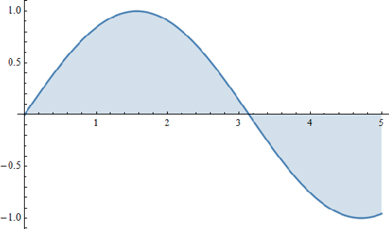
• Try to use any f[x] in the box above, for example Sin[x], and you will see how the next graph is updated. The process will repeat itself anytime you write a new function in the box.

  Dynamic[Plot [a, {x, 0, 5}, Filling → Axis]]

  

1.4.5 List and Matrices

Lists (List) are a fundamental concept in Mathematica. Lists or domains are written inside curly brackets with the elements separated by commas: {a, b, c}. For a description of list operations see the documentation: guide/ListManipulation. We’ll describe them in more detail in later chapters.

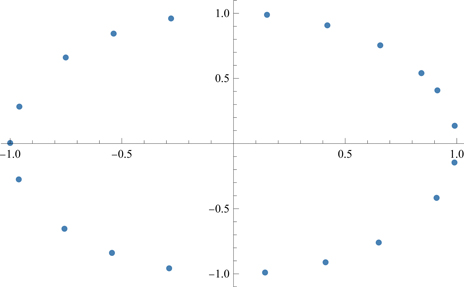
• In the example below we generate a list with Table.

  list1 = Table[{Sin[n], Cos[n]}, {n, 20}];

• We see that these are pairs of numbers corresponding to an ellipse that we can use to represent it graphically.

  ListPlot[list1]

  

Matrices have list format and consist of lists of sublists.

• Let’s create a matrix of random numbers.

  mat = RandomInteger[10, {5, 5}];

• We add InputForm so you can see the output displayed in the internal format used by Mathematica.

  mat // InputForm
  
  {{4, 6, 3, 9, 8}, {3, 7, 0, 8, 6}, {5,
  6, 10, 8, 10}, {3, 1, 10, 3, 8}, {0, 5,
  0, 4, 5}}

• If desired, matrices can be presented in standard mathematical notation.

  MatrixForm[mat]

  (4639837086561081031103805045)

• Since they are lists, matrices can be handled as such. For example, here we extract the second element of the first sublist:

  mat [[1, 2]]

  6

For further details about matrix operations you can consult the documentation: guide/MatrixOperations.

1.4.6 Graphics

One of the most remarkable aspects of Mathematica is its graphical capabilities. The program’s tool for 2D graphics can be accessed by pressing or by selecting in the menu bar Graphics ▶ Drawing Tool.

The most commonly used functions to represent graphics are Plot, Plot3D and ListPlot, of which we have already seen some examples. However, there are many more.

• Since Mathematica 9, when typing Plot the context-sensitive input assistant will show you all the words that include the word Plot, browse them. Alternatively type the following command and execute it (its output is omitted):

  ?*Plot*

The names that are shown can give you a hint about the type of plot they generate. Click on the chosen name to get more detailed information. In some cases you will be referred to the plot options.

• The graphical functions don’t end there. The ones that include the word Chart are usually related to statistical graphs. Similarly to the previous case you can use the command:

  ?*Chart*

• Graphics-related functions include numerous options, as you can see in the case of Plot. Use the following command (its output is omitted):

  Options[Plot3D]

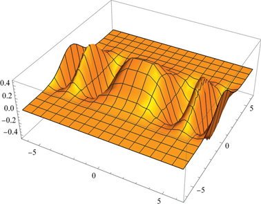
• The next cell displays the surface cos(x) sin(y) bounded by the ring 3 ≤ x² + y² ≤ 30. Note that to set the region where the function exists we use the RegionFunction option.

  Plot3D[Cos[x]Sin[y], {x, -2π, 2π},
   {y, -2π, 2π}, RegionFunction → (3 ≤ #1² + #2² ≤ 30 &),
   BoxRatios → Automatic, PlotStyle → Blue, ImageSize → Small]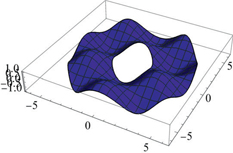

  

You can interact with 3D graphics: Click on the graph and you’ll see that you can rotate it, with click you can zoom, and with click you can move it around.

• The code below generates the famous Lissajous curves. Using Grid we can show a two-dimensional mesh of objects, in this case graphs. We also use the Tooltip function to display labels related to objects (not only graphics) that will be shown when the mouse pointer is in the area of such objects. Here, when the mouse pointer hovers over the chosen curve, you’ll see the function that generated it.

  Grid[Table[Tooltip[ParametricPlot[{Sin[nt], Sin[mt]}, {t, 0, 2Pi},
   ImageSize → 70, Frame → True, FrameTicks → None, Axes → False],
   {Sin[n t], Sin[m t]}], {m, 3}, {n, 3}]]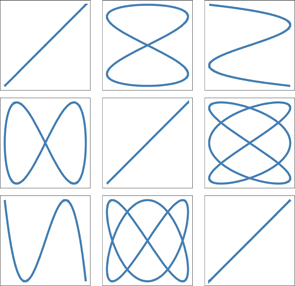

  

Other functions that do not include Plot or Chart but that are also useful for creating graphs are Graphics, Graphics3D and ColorData, as the following example shows.

• Representation of the water molecule.

  Graphics3D[{Specularity[White, 50], ColorData["Atoms", "H"],
   Sphere[{0, 0, 0}, .7], Sphere[{1.4, 0, 0}, .7], ColorData["Atoms", "O"],
   Sphere[{.7, 0, .7}]}, Lighting → "Neutral", ImageSize → Small]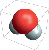

  

If you want to learn more about graphics, you can select the text with the cursor and press <F1>. For example: Select the text shown below and press <F1>:

tutorial/GraphicsAndSoundOverview

Graphics can be completed with legends using PlotLegends (if you are using a version prior to Mathematica 9 you will need to first execute Needs [“PlotLegends`”])

• In the following example we use AxesLabel to add labels to the axes and PlotLegends → “Expressions” to show the represented functions.

  Plot[{Sin[x], Cos[x], Tan[x]}, {x, 0, 2 Pi},
   AxesLabel → {"x", "f(x)"}, PlotLegends → "Expressions"]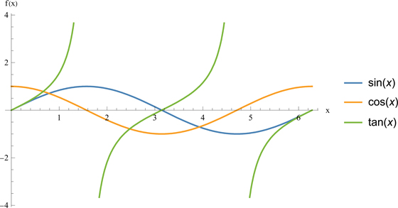

  

1.4.7 Images

Image processing has also experienced a significant improvement in the most recent versions of Mathematica. Starting with Mathematica 9, when clicking on an image you will see a menu with numerous options (Figure 1.12).

• The following command loads an image so we can play with it.

  ExampleData[{"TestImage", "Lena"}]

  

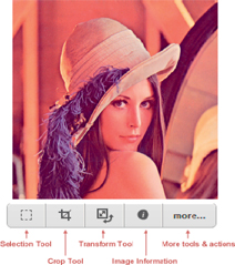
  Figure 1.12     The Image Assistant.

• Since version 9, a row of icons, the Image Assistant, appears below the image. Click on any of them. For example, after clicking on more... the following menu (Figure 1.13) will be deployed:

  

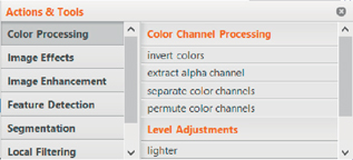
  Figure 1.13     Additional capabilities available from the “more... option” in the Image Assistant.

• Play with the controls. When you click on one of them, a miniature version of the image will be shown where you will be able to check the effect on the original image. For example: When clicking on invert colors you’ll see Figure 1.14.

  

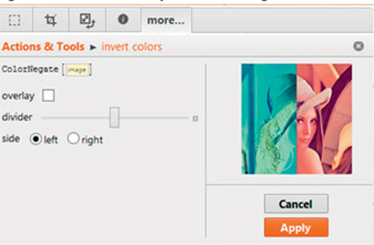
  Figure 1.14     Inverting the colors using the Image Assistant.

After getting the desired effect press Apply and the change will be applied to the image. An alternative way is to copy the command that appears in the menu: ColorNegate[image] to obtain the same result. Copy it to an input cell and execute it. This last procedure is the appropriate one if you want to create a program or explain how the image has been modified. We will be using this method when we refer to image processing in later chapters.

1.4.8 Manipulate

Among the improvements in the most recent versions of Mathematica is the addition of instructions to enable dynamic and interactive operations. One of the most significant examples of this is the Manipulate command, as can be seen in the following examples.

• Type the command shown below. Note how sliders are created for each of the parameters being defined. Click on the symbol included in the output to show the buttons created by Manipulate.

  Manipulate[Plot[Sin[frequency x + alpha], {x, -2π, 2π},
   ImageSize -> Small], {frequency, 1, 5}, {alpha, 0, Pi/2}]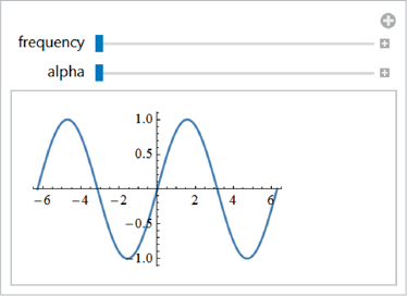

  

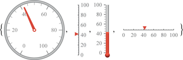
In the previous example we have used the ImageSize → Small option for printing purposes. We will use the option throughout the book but if you repeat the example in your computer you can ignore it.

1.4.9 Gauges

Since Mathematica 9 different types of gauges have been included that can behave dynamically and be customized:

Through[{AngularGauge, VerticalGauge, ThermometerGauge, HorizontalGauge}[
  42, {0, 100}, ImageSize → Tiny]]

1.4.10 Handwritten Text Recognition

Among the latest new features is the inclusion of machine learning functions. Let’s see an example.

• Handwrite different numbers on a white piece of paper, scan them or type them in a touch screen (in MS Windows you can use the Crop application) and establish their equivalence as shown in the next function.

  

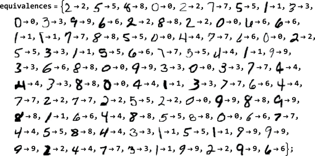
• Use the command Classify to establish equivalences based on the examples. Note that for a given number, its handwritten equivalent may not be the same. This function uses statistical criteria to assign a weight to each established equivalence.

  digits = Classify[equivalences]

  

• Copy from above the numbers 0 to 10 in a list like the following:

  

  {0, 1, 2, 3, 4, 5, 4, 7, 8, 9}

• Note that the identification has been done correctly except in the case of 6 that has been mistaken with 4. The program assigns probabilities based on the stored data. You can check that the probability assigned to the symbol is higher for 4 than for 6. Even a person may not be sure whether the handwriting represents a 6 or a 4.

  

  {4 → 0.375915, 6 → 0.354657, 0 → 0.235305}

• If 6 is written in a less equivocal way the probability of a correct identification improves substantially.

  

  {6 → 0.992954}

1.4.11 Things to Consider

Don’t forget that for everything to work correctly, it’s necessary that all the commands in the same session are executed sequentially. Cells are executed based on the order of evaluation and not on the order they are shown on the screen. This means that if a function calls previous functions, those functions should have been executed in advance. It’s not enough to see them already typed. If you modify an assignment that is used in a later function, you will have to execute again all the related cells.

• Execute sequentially the following three cells:

  a = 3 (*first*)

  3

  b = x^a (*second*)

  x³

  a b (*third*)

  3x³

Now type a = 2 in the first cell. Execute it and then the third one (a b) What has happened?

Mathematica retains information about all the variables defined in a session, even after starting a new notebook. Because of that, when starting a new section that will not be using the variables previously defined it would be a good idea to clear them first.

• One way to remove all the values and definitions is as follows:

     Clear ["Global`*"]

Another way to achieve the previous result is to limit the application of the variables to a certain context through the menu bar: Evaluation ▶ Notebook Default Context. This offers the possibility to limit the defined variables to the active notebook or to certain cells grouped following a specific criterion, for example: all the cells belonging to the same section. As a matter of fact this chapter has been created using this option. The input counter will reset itself when a new group of cells is created (here it cannot be seen because we have suppressed the symbol In[n]=). Nevertheless, this method is less straightforward than Clear [“Global` *”]. We should evaluate the most appropriate way based on the situation.

If you really want to remove all the information and not only the variables, the best way is to quit the session. This requires that you exit Mathematica (actually it requires that you exit the program Kernel). You can do that in several ways: With File ▶ Exit or if you don’t want to exit the notebook use either Evaluation ▶ Quit Kernel or in an input cell type Quit[]. Once you have exited, the program removes from memory all the assignments and definitions. When you execute the next command the kernel will be loaded again.

Although Mathematica tries to maintain compatibility with notebooks created in previous versions, the compatibility is not always complete so you may have to make some modifications. When you open a notebook created in a previous Mathematica version for the first time, the program will offer you the possibility of checking the file automatically; Accept it and read the comments that you may receive carefully. In many cases Mathematica will modify expressions directly and let you know about the changes made giving you the option to accept or reject them. In other cases it will offer suggestions.

Remember: If you don’t understand a function use the Documentation Center.

1.5 Computational Capabilities

Early versions of Mathematica were mainly oriented toward symbolic computations. However, the latest versions of the program, apart from having significantly increased those capabilities, have complemented them with powerful functions for numeric calculations. An example of this combination is the large collection of probability related functions that provide seamlessly either symbolic or numeric answers depending on the inputs.

1.5.1 Equation Solving

We are going to show several available functions for solving different types of equations. In the examples we will use only one variable but the same functions can be used with a higher number of variables. Don’t forget to use “==” to indicate equality in an equation.

• It is interesting to compare Solve and Reduce.

  Solve[{x + ay + 3z == 2, x + y - z == 1,
  2x + 3y + az == 3}, {x, y, z}]

  {{x→1,y→−1−a−3,z→−1−a−3}}

• Reduce generates all the solutions depending on the value of the parameter a and uses a more formal notation in its output.

  Reduce[{x + ay + 3z == 2, x + y - z == 1,
  2x + 3y + az == 3}, {x, y, z}]

  (a=2∧y=15(5−4x)∧z=x5)∨(a−2≠0∧x=1∧a+3≠0∧y=1a+3∧z=y)

• Reduce and Solve accept constraints regarding the variables domain.

  Reduce[272x-1x==92x−1,x,Reals]x=12∨x=3

• Solve can solve geometrically formulated problems. In this case the solution to the intersection of a line passing through the points {0,0},{2,1}, with a circumference of radius r = 1 centered at {0, 0}(Mathematica uses Circle to refer to the circumference and Disk to refer to the circle, by default the commands assume a circle or circumference of r = 1, and centered at {0, 0}):

  Solve[{x, y} ∈ InfiniteLine[{{0, 0}, {2, 1}}] && {x, y} ∈ Circle[], {x, y}]

  {{x→−25,y→−15},{x→25,y→15}}

  Graphics [{{Blue, InfiniteLine[{{0, 0}, {2, 1}}], Circle[]},
    {Red, Point [{x, y}] / . %}}]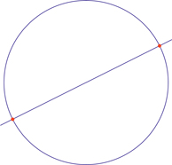

  

An analytical solution may not exist in many cases or we may be interested in a numeric result. In those situations we can use FindRoot or NSolve.

• With FindRoot you must define, for a given equation, the variable whose value you want to find and an initial starting point at which the search for the solution starts.

  FindRoot [Cos[x] == x + Log[x], {x, 1}]

  {x → 0.840619}

  NSolve [x^5 − 6 x^3 + 8x + 1 == 0, x]

  {{x → −2.05411}, {x → −1.2915}, {x → −0.126515}, {x → 1.55053}, {x → 1.9216}}

1.5.2 Integration

• The symbolic integration capabilities of Mathematica are very powerful as shown in the example below.

  Integrate[Exp[1 - x^2], x]

  12eπ erf(x)

• However, there are times when symbolic integration is not possible and is necessary to integrate using numerical methods (Log refers to the base logarithm, to indicate the base 10 logarithm type Log[10, expr]).

  NIntegrate[Log[x + Sin[x]], {x, 0, 2}]

  0.555889

• It is also possible to limit the integration to a certain region by using the Boole function. In this example this region is a cone with radius 1.

  Integrate[(x² + y²) Boole[0 ≤ z ≤ 1 && x² + y² ≤ z²],
    {x, -1, 1}, {y, -1, 1}, {z, 0, 1}]

  π10

• With RegionPlot we can represent the integration region, a feature that from an educational point of view may be of interest.

  RegionPlot3D[0 ≤ z ≤ 1 && x^2 + y^2 ≤ z^2,
   {x, -1, 1}, {y, -1, 1}, {z, 0, 1}, ImageSize → Small]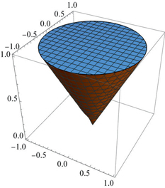

  

We can even specify assumptions, with Assumptions, about the parameters of the function that we wish to integrate.

• In this example we specify that when integrating xⁿ, n is greater than 1.

     Integrate[x^n, {x, 0, 1}, Assumptions -> n > 1]

  1n+1

• We can also integrate over a region. In this example, over a sphere centered at {0,0,0} and with radius r>0. Obviously, we are calculating the volume of the sphere.

     Integrate[1, {x, y, z} ∈ Ball[{0, 0, 0}, r], Assumptions -> r > 0]

  4 π r33

1.5.3 Sums, Logical Operations, Simplifications and Differential Equations

• We can evaluate sums and products with finite and infinite terms.

  Σk=1∞1K6π6945

• We can also perform logical operations.

  Log[2]<1.4<2

  True

• To check whether two expressions are equivalent “===” can be used. Note that 3 y 3.0 in Mathematica are different numbers.

  1 === 3/3

  True

  1 === 3.0/3

  False

• Next, we solve a differential equation for a pendulum with damping constant k. Using Manipulate we can make the value of k vary from 0 to 3 and plot the solution. By using Evaluate we are forcing Mathematica to solve the differential equation first, and then substitute x and k with the given values. Note that the use of the pattern “y[x]/. something”. “ /.” means “replace with” (in the example: y[x] is replaced by the equation solution).

  Manipulate[Plot[Evaluate[y[x] / .
      DSolve[[y″[x] + k y′ [x] + 40 y[x] == 0, y[0] == 1, y'[0]==13}, y[x], x]],
    {x, 0, 4}, ImageSize → Small], {k, 0, 3}]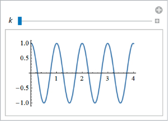

  

1.5.4 Application: The Lorenz System

There are many functions available for numerical methods, such as NDSolve, used when solving differential equations numerically.

• An example of the use of NDSolve is its application to the well-known Lorenz system, a simplified model to study atmospheric convection movements that exhibit chaotic behavior.

  eqs = {x'[t] == −3 (x[t] − y[t]),
      y'[t] == -x[t] z[t] + 26.5x[t] - y[t], z'[t] == x[t] y[t] - z[t]};
  ics = {x[0] == z[0] == 0, y[0] == l};
  sol = NDSolve [{eqs, ics}, {x, y, z}} {t, 0, 200}, MaxSteps -> ∞]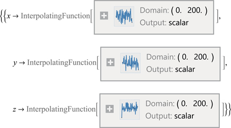

  

• The solution to the previous equation in the phase space is displayed using ParametricPlot3D.

  ParametricPlot3D[{x[t], y[t], z[t]} /. sol[[1]], {t, 0, 200},
    PlotPoints → 1000, ColorFunction → (Hue[#4] &), ImageSize → Small]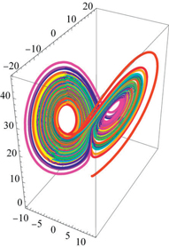

  

1.5.5 Statistical Calculations

Mathematica probably includes as many functions, if not more, than other specialized statistical software programs. The downside is that users must have a deep understanding of what they are trying to accomplish.

• This example shows the probability density function (pdf) and the cumulative density function (cdf) of a Poisson distribution with mean μ = 10. An option in PlotLegends is included to place the legend in the desired position.

  pdf = PDF[PoissonDistribution[μ], x]

  {e−μ μxx!x≥00True

  cdf = CDF[PoissonDistribution[μ], x]

  {Q([x]+1,μ)x≥00True

  DiscretePlot[Evaluate[{pdf, cdf} /. μ → 10], {x, 0, 15}, PlotRange → All,
    PlotLegends → Placed[{"Probability", "Cumulative Probability"}, Below]]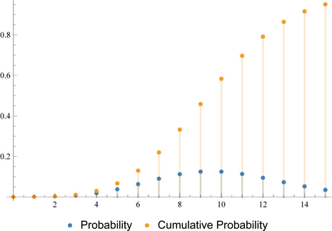

  

1.6 Utilities

1.6.1 Example Data

The installation of the program includes a set of files with data from different fields that can be used to test some of the functions. To download them use the command ExampleData.

• Let’s download the original text of Charles Darwin’s book On the Origin of Species:

  txt = ExampleData[{"Text", "OriginOfSpecies"}];

• To find out how many times the word “evolution” appears compared to the word

  “selection” we use the function StringCount, specifying the chosen word or text.

  StringCount[txt, "evolution"]

  4

  StringCount[txt, "selection"]

  351

1.6.2 Accessing External Data

One of the most important features of Mathematica since Version 8, already mentioned, is its integration with Wolfram|Alpha (tutorial/DataFormatsInWolframAlpha). This enables us to access information about practically anything and once downloaded it can be used in the Mathematica environment to perform further calculations.

• Type Japan vs. Germany. Several frames (pods) will be displayed, each of them containing information about an aspect of the question. In the right corner of each frame the symbol appears. Click on one of them and you will see a menu with several options. In this example, we chose the Geographic Properties frame and clicked on the Subpod content. The following entry was generated afterward:

  WolframAlpha["Japon vs. Germany",
   IncludePods → "GeographicProperties:CountryData",
   AppearanceElements → {"Pods"},
   TimeConstraint → {30, Automatic, Automatic, Automatic}]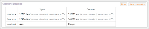

  

• We repeat the same steps for “China vs USA” but in this case instead of Subpod content we choose ComputableData. The output is shown below. This has the advantage of being generated as a list allowing easy subsequent manipulation.

  WolframAlpha["China vs USA",
   {{"GeographicProperties:CountryData", 1}, "ComputableData"}]

  (ChinaUnited Statestotal area9.597×106 km29.631×106 km2land area9.326×106 km29.162×106 km2continentAsiaNorth America)

In the WolframAlpha style you can select the information you are interested in by choosing from the menu that appears after clicking on ▶ Subpod content or ComputableData in the desired frame. An input will be generated to get only the desired information.

You can also access external data through Computable Data (guide/ComputableDataOverview), a group of functions specific to Mathematica, to obtain the desired information. We will cover them in more detail in Chapter 5.

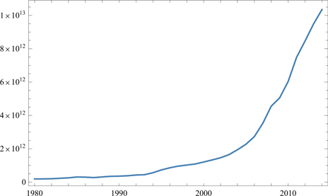
• The graph below shows the evolution of the gross domestic product, GDP, of China from 1980 to 2015.

  DateListPlot [CountryData["China", {{"GDP"}, {1980, 2015}}]]

  

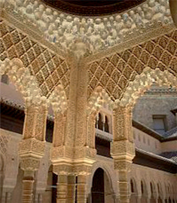
• We can even obtain information from Wikipedia using the new function (available since Mathematica 10.1): WikipediaData.

  WikipediaData["Alhambra", "ImageList"][[5]]

  

1.6.3 Application: Everybody Out

We would like to estimate the amount of energy required to move the entire population off-planet: https://what-if.xkcd.com/7/. Without considering the weight of the rockets, the idea is to see how we can solve this problem accessing external data from within Mathematica. The same approach can be useful to solve other types of problems.

The data that we need to know are: the kinetic energy equation (it’s been such a long time since we took high-school physics that we have forgotten it) and the values of its components. We will need to know the world population as well.

• The kinetic energy equation can be found using FormulaData.

  FormulaData["KineticEnergy"]

• Or the free-form input format: typing Kinetic Energy Equation.

  

  K=12 m v2

• From the equation we can see that we need to know: m (mass per person) and v (escape velocity from Earth). Both values can be obtained with the free-form input format typing: average adult weight and earth’s escape velocity or similar statements.

  

  82 kg

  

  1.118×10⁴ m/s

• With these data we obtain the energy per person. We need to multiply them by n, the world population.

  n = QuantityMagnitude[CountryData["World", "Population"]]

  7.13001 × 10⁹

• Now, after evaluating the kinetic energy equation, we get the necessary kinetic energy to put the entire world population in orbit. Naturally this is just a toy example that has nothing to do with reality since we would need to consider the mass of the launcher and the fact that people would have to go in spaceships that have masses much bigger than that of their passengers. Until now we have sent about 600 people into space. The trip in a Soyuz spacecraft costs about 20 million dollars per person. Multiply that figure by the number of people living on earth and the result is thousands of times bigger than the world’s GDP. Let’s hope that we will not need to put the entire human population into orbit!

  UnitSimplify[12 m v^2*n]

  3.65391 × 10¹⁹ J

1.6.4 Interactive Visualizations (Demonstrations)

In http://demonstrations.wolfram.com you can find thousands of small interactive applications of great educational value. In this book we’ll refer to them using the word “demonstrations”. If you don’t know how to build them just download and open the files; later on you’ll be able to modify them to suit your needs or even make new ones. In Chapter 4 we’ll learn how to create them.

• This example explores Coulomb’s law. This law describes the interaction between two charges (based on ‘Potential Field of Two Charges’ created by Herbert W. Franke: http://demonstrations.wolfram.com/PotentialFieldOfTwoCharges/).

  Manipulate[ContourPlot[q1/Norm[{x, y} - p[[1]]] + q2/Norm[{x, y} - p[[2]]],
    {x, 2, -2,}, {y, 2, -2}, Contours → 10],
   {{q1, - 1}, -3, 3}, {{q2, 1}, 3, -3},
   {{p, {{-1, 0}, {1, 0}}}, {-1, -1}, {1, 1}, Locator}, Deployed → True]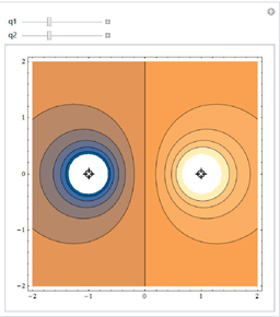

  

  Move the locators around with the mouse to see how the potential fields change.

1.6.5 Packages

Commands can be used directly or can be put together to develop applications for specific purposes (packages). The packages included in Mathematica can be seen in Documentation Center ▶ StandardExtraPackages and Documentation Center ▶ InstalledAddOns. StandardExtraPackages are the ones included in the program installation. Many of those functions now in the packages will probably be part of the kernel of the program in the future.

Installed AddOns are packages developed by users for specific purposes. Some of them are available in http://library.wolfram.com/infocenter. This book's author has developed several packages, some of them available in http://diarium.usal.es/guillermo.

Normally these packages will be copied in Addons/Applications, located in the Mathematica installation directory.

To load a package you can type Needs[“package name`”] or <<package name`. For example, the following package includes various functions related to the properties of the radiation emitted by a black body.

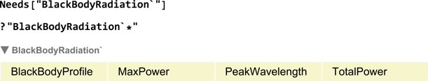
• The following package function calculates the peak wavelength of a black body for a given temperature.

  PeakWavelength[5000 Kelvin]

  5.79554 × 10⁻⁷ Meter

In a later chapter we’ll give a brief introduction to package development.

1.7 Editing Notebooks

We’ve seen that the interaction with Mathematica is done through the Front End (what we usually see when using Mathematica), and this generates files named "Mathematica notebooks". What you are currently reading is one such notebook.

Each Mathematica notebook (file.nb) is a complete and interactive document containing text, tables, graphics, calculations and other elements. The program also enables high-quality editing so notebooks can be ready for publication (some journals directly admit papers in nb format).

1.7.1 Notebook Structure

Each cell has a style. For example, the previous cell has the style Subsection associated to it. To do that we just need to select its cell marker (]) and in the style box choose Subsection.

Notebooks are organized automatically into a hierarchy of different cell types (title, section, input, output, figures, etc). If you click on the exterior cell marker, the cells will be grouped. For example, if you click on a section, all the cells associated to that section will collapse and you will only see the title of the section. You just need to click again to see them back.

This is an ordinary text with the color formatted Format ▶ Text Color.

Click on a text cell and modify its format.

With Insert ▶ Hyperlink we can create hyperlinks to jump from one location to another inside the same notebook, to another notebook or to an external link.

Using Format ▶ Text Color we can choose the font, face, size, color, etc. We can even use special characters such as .

This notebook, like any other, has a predefined style. The style tells Mathematica how to display its contents. There are many such styles. To choose the notebook’s overall style you can use Format ▶ Stylesheet. With Format ▶ Style you can define the style of a particular cell. Additionally, inside a style, we can choose the appropriate working environment Format ▶ Screen Environment. Try changing the appearance of a notebook by modifying the working environment.

1.7.2 Choosing Your Style

To edit an article, book or manual the Writing Assistant palette is of great help. Load it. Note that is divided into three sections: Writing and Formatting,Typesetting and Help and Settings. See the help included in the palette.

If you click inside the palette on the button Stylesheet Chooser... (alternatively you can go to Format ▶ Stylesheet ▶ Stylesheet Chooser...) a separate window with icons representing different styles will appear (Figure 1.15). If you press on the upper part of any of the icons (New) a new sample notebook formatted according to that style will be generated. You will be able to use it and modify its contents to suit your needs. If you click on the bottom part of the icons (Apply), the style will be applied to the currently active notebook. For example, in the next screenshot (Figure 1.15), by clicking on the upper part of the Textbook icon, a notebook with a Textbook template style will be opened.

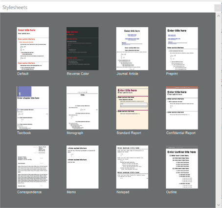
Figure 1.15     The Stylesheet Chooser.

When a new cell is created, depending on the stylesheet, by default it will be of a certain format type, for example with the Default stylesheet new cells are of type Input.

When typing in a new notebook choose the stylesheet from the beginning with Format ▶ Stylesheet ▶ Stylesheet Chooser... . After clicking on the upper side of the icon representing the desired style (New), you will be able to use and modify the template according to your needs.

1.7.3 Typesetting Advice

If you are interested in emphasizing text containing formulas using classical mathematical notation, begin by typing in a text cell. Select the formula and define it as Inline Math Cell by pressing or, in the Writing Assistant palette, choose Math Cells ▶ Inline Math Cell. Finally, in the same palette in Cell Properties click on Frame and select the appropriate one . That’s how the following example was done:

¿What is the domain of the function f(x)=x2−1?

If you’d like to type a sequence of formulas and align them at the equal signs, in Writing Assistant, choose Math Cells ▶ Equal Symbol Aligned Math Cell.

Figure 1.16     Aligning equations at the equal sign.

Sometimes it may be useful to type both, the formula and its result, as part of the text. This can be done by writing and executing the function in the same text cell. For example: using a palette write ∫x³ dx = ∫x³ dx. Now select the second term of the equation and press . Or, in the menu bar, choose Evaluation ▶ Evaluate in place, and the previous expression will become ∫x3dx=x44.

When creating a document, you may be interested in seeing only the result. In that case you can hide the Input cell.

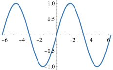
• To hide the input just click directly on the output marker cell. The following example was created by executing Plot[Sin[x], {x, -2 Pi, 2 Pi}] and then hiding the command to display only the graph.

  

All Mathematica commands are in English but the menus and palettes can also be displayed in any of the additional 12 languages offered since version 11. The alternatives include Chinese, French, German, Italian, Japanese, Korean and Spanish among others. Users can take advantage of this functionality by going to Edit ▶ Preferences ▶ Interfaces. Once an option different from English is selected, every function will be automatically annotated with a “code caption” in the chosen language. Mathematica 11 also includes a real-time spell checker that works with any of the supported languages. Alternatively, users of previous Mathematica versions can review the English contents of a notebook with Edit ▶ Check Spelling....

With Edit ▶ Preferences and with Format ▶ Option Inspector (see tutorial/OptionInspector) you will be able to customize many features of Mathematica that can be applied globally, to a notebook or to a particular cell. For example: with Format ▶ Option Inspector ▶ Global Options ▶ File Locations you can change Mathematica default directories.

1.7.4 The Traditional Style

We’ve seen that Mathematica by default uses the style: StandardForm in the input cells (Input) by default. However, if we’d like to create better looking documents, it’s recommended to use the TraditionalForm style that is similar to the one used in traditional mathematical notation.

If the main purpose of a document is to be read by others, it may be convenient to present the inputs and outputs using the traditional notation. It’s likely that the reader will not realize that it was created with Mathematica. This is specially true if the document is saved using the cdf format to which we will refer in the following section.

You can write your inputs in StandardForm. Once you verify that they work you can convert them to the traditional style.

• Example: Let’s type:

  Limit[(x + Δx)2−x2Δx,Δx→0]2x

• We convert the cell to the traditional form by selecting it and clicking on: Cell ▶ Convert to ▶ TradicionalForm. Then the cell above will be shown as follows:

  limΔx→0(x+Δx)2−x2Δx2x

If an entry is in the traditional style, to see how it was originally typed convert it to the standard style by selecting the cell and choosing from the menu bar Cell ▶ Convert to ▶ StandardForm.

We can make an output to be shown in the traditional form by adding // TraditionalForm at the end of each input. There are several ways to apply this style to all the outputs in a notebook. In Edit ▶ Preferences ▶ Evaluation you can specify for all the outputs to be displayed in the traditional form (TraditionalForm). Another easy one is to use the following command:

   SetOptions[EvaluationNotebook[],
    CommonDefaultFormatTypes -> {"Output" -> TraditionalForm}]

It’s recommended to include the command above in a cell at the end of the notebook and define it as an initialization cell (click on the cell marker and check Cell ▶ Cell Properties ▶Initialization Cell). This way, the cell will be executed before any other cell.

In many of the styles available in Stylesheet Chooser... outputs are displayed using the standard form. In this chapter we have used a customized stylesheet that shows outputs in the traditional format. In the rest of the book, we will almost always use the standard form since what we are trying to highlight is how to create functions with Mathematica and for that purpose the classical format is not adequate.

1.7.5 Automatic Numbering of Equations and Reference Creation

Textbook and scientific articles frequently use numbered equations. This can be done as follows:

• First open a new notebook (File ▶ New ▶ Notebook) and select one of the stylesheets available in the format menu. For instance Textbook: Format ▶ Stylesheet ▶ Book ▶ Textbook

• Then create a new cell and choose EquationNumbered as its style (Format ▶ Style ▶ EquationNumbered). The cell will be automatically numbered, then you can write the equation, for example: a + b = 1.

a+b=1(1.1)

If you have opened a new notebook using the Textbook style, you will probably see (0.1) instead of (1.1). It’s possible to modify the numbering scheme but it is beyond the scope of this chapter. When you need to number equations, sections, and so on, remember that it is a good idea to select the stylesheet directly from the Writing Assistant palette: Palettes ▶ Writing Assistant ▶ Stylesheet Chooser... . After selecting Textbook (New), a new notebook will be generated with many different numbered options such as equations, sections, etc. You can then use that notebook as a template.

If you wish to insert an automatic reference to the equation proceed as follows:

• Write an equation in a cell with the EquationNumbered style. Then go to Cell ▶ Cell Tags ▶ Add/Remove... and add a tag to the formula. Let’s give it the tag: “par” (we write “par”, from parabola, although we could have used any other name). A good idea would be also to go to Cell ▶ Cell Tags and check ▶ Show Cell Tags, keeping it checked while creating the document, and only unchecking it after we are done. This will enable us to see the cell tags at all times. The first equation done this way is written below:

par

x2=1(1.2)

• If you wish to refer to this equation: Type the following: (1. ), put the cursor after the dot and go to Insert ▶ Automatic Numbering. In the opening dialog (Figure 1.17) scroll down to EquationNumbered and choose the tag of the equation, in our case: “par” then press OK (see the screen below). After this has been done the number of the equation appears between the parentheses: (1.2). If you click on the “2” the cursor will go immediately to the actual equation.

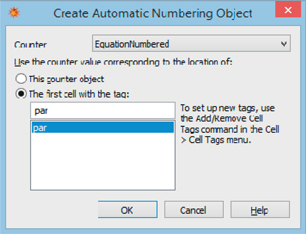
Figure 1.17     Creating an automatically numbered object.

1.7.6 Cell Labels Display

As we have mentioned previously, any time we execute an input cell, a label in the form In[n] is shown, but we can choose not to display it. This can be done from Edit ▶ Preferences or typing SetOptions[SelectedNotebook[], ShowCellLabel → False]. You can also reset the counter (set In[n] to 1) in the middle of a session by typing the following in an input cell: $Line=1.

1.8 Sharing Notebooks

1.8.1 Save as...

Documents created with Mathematica are saved with extension *.nb, Mathematica’s own format, by default. If you share any of these documents with someone, that person will require access to Mathematica.

However, Mathematica can also save documents in other formats. To do that, in the menu bar, choose File ▶ Save As ▶. Then, from the list of options, select the desired one.

Very often we may be interested in saving a document in pdf format to reach a broad audience. We can also use TeX (widely used in professional journals in mathematics) or HTML/XML if we want to use it in a website. Probably it would be better to save the web files in XML since everything can be included in a single file in contrast to HTML, where there is a main file and numerous additional files associated to it. However, if we’d like to keep Mathematica’s interactive capabilities the most appropriate format would be cdf (Computable Document Format).

1.8.2 The Computable Document Format (*.cdf)

As previously discussed, if you’d like other people without access to Mathematica to read your documents without losing their interactivity, you should save them in the cdf format: File ▶ CDF Export ▶ Standalone or File ▶ Save As ▶ Computable Document (*.cdf).

The main advantage of this format is that it keeps the interactivity of the objects created with Manipulate. In this case your documents can be read with the Wolfram CDF Player (available for download for free from http://www.wolfram.com/cdf-player). When sharing a cdf file, to ensure that the intended reader can open it, we recommend that when sending it the link above is included as well.

You can also create a cdf file (normally a section of a notebook) to be embedded in a web page. In the menu bar, select File ▶ CDF Export ▶ Web Embeddable.

For more detailed information see in the help system: "Interactivity in .cdf Files" or, even better, visit: http://www.wolfram.com/cdf.

The Wolfram CDF Player is not just a reader of Mathematica documents for users without access to the program. The player can also avoid displaying the functions used in the inputs showing only the outputs (remember the trick that we have seen previously to hide the inputs and only show the outputs). Furthermore, it can include dynamic objects created with Manipulate so that readers can experiment with changing certain parameters and visualizing the corresponding effects in real time. Additionally, readers will not even know that the original document was generated in Mathematica. To see all these capabilities in action take a look at the following cdf document:

http://www.wolfram.com/cdf/uses-examples/BriggsCochraneCalculus/BriggsCochraneCalculus.cdf

Many of the Wolfram Research websites, such as Wolfram|Alpha (http://www.wolframalpha.com), allow visitors to generate and download documents in cdf format. The same happens with the Wolfram Demonstrations Project (http://demonstrations.wolfram.com) where the files are available in cdf format and you can download and run them (for example, in a digital board connected to a PC with the Wolfram CDF Player).

1.9 The Wolfram Cloud

As stated at the beginning of the chapter, the program can be executed in the cloud, that is: in a server accessible through the Internet using a browser, in what is known the Wolfram Cloud (http://www.wolframcloud.com/). The Wolfram Cloud can also be used to store files remotely, as a matter of fact all the files generated locally are interchangeable with the cloud-generated ones. If you don’t have access locally and you would like to start familiarizing yourself with Mathematica you can do so directly using the Wolfram Development Platform, part of the Wolfram Cloud, for free. If you are planning to use this option heavily, the cost will depend on your requirements and whether you already own a Mathematica license or not. In any case, you must register as a user using a Wolfram ID.

If you already registered in the user portal https://user.wolfram.com, mentioned previously, you can use the same Wolfram ID. After signing up you can access the development platform by visiting http://www.wolframcloud.com and then clicking on the Wolfram Development Platform icon (http://develop.wolframcloud.com/app).

After entering your Wolfram ID and password, the screenshot shown in Figure 1.18 will appear although you might see an initial screen that is somewhat different since the Wolfram Cloud is constantly evolving.

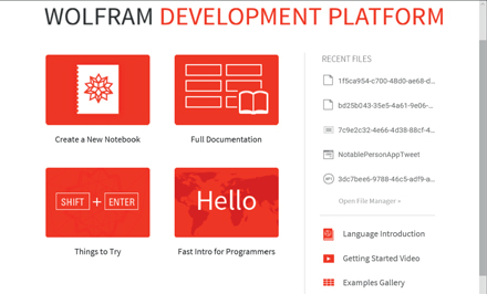
Figure 1.18     Welcome Screen in the Wolfram Development Platform.

You can now create a new notebook by clicking on: Create a New Notebook, and be able to reproduce most of the examples discussed in the chapter. You can also save the notebook in Wolfram Cloud, and when accessing it again, no matter from what location, you will be able to continue working on it. Additionally, you will have the possibility of accessing cloud files from a local Mathematica installation: File ▶ Open from Wolfram Cloud... or File ▶ Save to Wolfram Cloud... . Mathematica has specific functions related to the Wolfram Cloud. In later chapters we will refer to them. You can get an idea by clicking on: Getting Started... and watching the short video.

1.10 Additional Resources

To access the following resources, enter the web addresses in a browser:

An Elementary Introduction to the Wolfram Language by Stephen Wolfram is in Help ▶Wolfram Documentation ▶ Introductory Book ≫, or free on the web: http://www.wolfram.com/language/elementary-introduction/ (there is also a print version). Complete program documentation: http://reference.wolfram.com/language/

Explanatory video guides: http://www.wolfram.com/broadcast

Introductory program tutorials: http://reference.wolfram.com/language/tutorial/IntroductionOverview.html

Interactive applications: http://demonstrations.wolfram.com

Mathematics reference website: http://mathworld.wolfram.com/

Paid and free courses: http://www.wolfram.com/training/courses/

Information about the Computable document format (CDF): http://www.wolfram.com/cdf

News and ideas: http://blog.wolfram.com

Author’s website: http://diarium.usal.es/guillermo