
In 1938, a monograph entitled The Wave Principle was the first published reference to what has come to be known as the Elliott Wave Principle. The monograph was published by Charles J. Collins and was based on the original work presented to him by the founder of the Wave Principle, Ralph Nelson (R.N.) Elliott.
Elliott was very much influenced by the Dow Theory, which has much in common with the Wave Principle. In a 1934 letter to Collins, Elliott mentioned that he had been a subscriber to Robert Rhea’s stock market service and was familiar with Rhea’s book on Dow Theory. Elliott goes on to say that the Wave Principle was “a much needed complement to the Dow Theory.”
In 1946, just two years before his death, Elliott wrote his definitive work on the Wave Principle, Nature’s Law—The Secret of the Universe.
Elliott’s ideas might have faded from memory if A. Hamilton Bolton hadn’t decided in 1953 to publish the Elliott Wave Supplement to the Bank Credit Analyst, which he did annually for 14 years, until his death in 1967. A.J. Frost took over the Elliott Supplements and collaborated with Robert Prechter in 1978 on the Elliott Wave Principle. Most of the diagrams in this chapter are taken from Frost and Prechter’s book. Prechter went a step further and in 1980 published The Major Works of R.N. Elliott, making available the original Elliott writings that had long been out of print.
There are three important aspects of wave theory—pattern, ratio, and time—in that order of importance. Pattern refers to the wave patterns or formations that comprise the most important element of the theory. Ratio analysis is useful in determining retracement points and price objectives by measuring the relationships between the different waves. Finally, time relationships also exist and can be used to confirm the wave patterns and ratios, but are considered by some Elliotticians to be less reliable in market forecasting.
Elliott Wave Theory was originally applied to the major stock market averages, particularly the Dow Jones Industrial Average. In its most basic form, the theory says that the stock market follows a repetitive rhythm of a five wave advance followed by a three wave decline. Figure 13.1 shows one complete cycle. If you count the waves, you will find that one complete cycle has eight waves—five up and three down. In the advancing portion of the cycle, notice that each of the five waves are numbered. Waves 1, 3, and 5—called impulse waves—are rising waves, while waves 2 and 4 move against the uptrend. Waves 2 and 4 are called corrective waves because they correct waves 1 and 3. After the five wave numbered advance has been completed, a three wave correction begins. The three corrective waves are identified by the letters a, b, c.
Along with the constant form of the various waves, there is the important consideration of degree. There are many different degrees of trend. Elliott, in fact, categorized nine different degrees of trend (or magnitude) ranging from a Grand Supercycle spanning two hundred years to a subminuette degree covering only a few hours. The point to remember is that the basic eight wave cycle remains constant no matter what degree of trend is being studied.
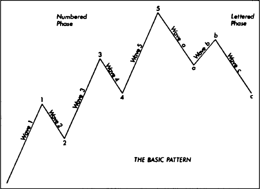
Figure 13.1 The Basic Pattern. (A.J. Frost and Robert Prechter, Elliott Wave Principle [Gainesville, GA: New Classics Library, 1978], p. 20. Copyright © 1978 by Frost and Prechter.)
Each wave subdivides into waves of one lesser degree that, in turn, can also be subdivided into waves of even lesser degree. It also follows then that each wave is itself part of the wave of the next higher degree. Figure 13.2 demonstrates these relationships. The largest two waves—1 and 2—can be subdivided into eight lesser waves that, in turn, can be subdivided into 34 even lesser waves. The two largest waves—1 and 2—are only the first two waves in an even larger five wave advance. Wave 3 of that next higher degree is about to begin. The 34 waves in Figure 13.2 are subdivided further to the next smaller degree in Figure 13.3, resulting in 144 waves.

Figure 13.2 (Frost and Prechter, p. 21. Copyright © 1978 by Frost and Prechter.)
The numbers shown so far 1,2,3,5,8,13,21,34,55,89,144—are not just random numbers. They are part of the Fibonacci number sequence, which forms the mathematical basis for the Elliott Wave Theory. We’ll come back to them a little later. For now, look at Figures 13.1-13.3 and notice a very significant characteristic of the waves. Whether a given wave divides into five waves or three waves is determined by the direction of the next larger wave. For example, in Figure 13.2, waves (1), (3), and (5) subdivide into five waves because the next larger wave of which they are part—wave 1—is an advancing wave. Because waves (2) and (4) are moving against the trend, they subdivide into only three waves. Look more closely at corrective waves (a), (b), and (c), which comprise the larger corrective wave 2. Notice that the two declining waves—(a) and (c)—each break down into five waves. This is because they are moving in the same direction as the next larger wave 2. Wave (b) by contrast only has three waves, because it is moving against the next larger wave 2.
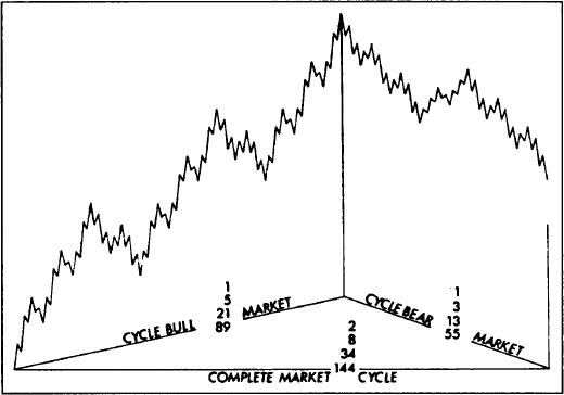
Figure 13.3 (Frost and Prechter, p. 22. Copyright © 1978 by Frost and Prechter.)
Being able to determine between threes and fives is obviously of tremendous importance in the application of this approach. That information tells the analyst what to expect next. A completed five wave move, for example, usually means that only part of a larger wave has been completed and that there’s more to come (unless it’s a fifth of a fifth). One of the most important rules to remember is that a correction can never take place in five waves. In a bull market, for example, if a five wave decline is seen, this means that it is probably only the first wave of a three wave (a-b-c) decline and that there’s more to come on the downside. In a bear market, a three wave advance should be followed by resumption of the downtrend. A five wave rally would warn of a more substantial move to the upside and might possibly even be the first wave of a new bull trend.
Let’s take a moment here to point out the obvious connection between Elliott’s idea of five advancing waves and Dow’s three advancing phases of a bull market. It seems clear that Elliott’s idea of three up waves, with two intervening corrections, fits nicely with the Dow Theory. While Elliott was no doubt influenced by Dow’s analysis, it also seems clear that Elliott believed he had gone well beyond Dow’s theory and had in fact improved on it. It’s also interesting to note the influence of the sea on both men in the formulation of their theories. Dow compared the major, intermediate, and minor trends in the market with the tides, waves, and ripples on the ocean. Elliott referred to “ebbs and flows” in his writing and named his theory the “wave” principle.
So far, we’ve talked mainly about the impulse waves in the direction of the major trend. Let’s turn our attention now to the corrective waves. In general, corrective waves are less clearly defined and, as a result, tend to be more difficult to identify and predict. One point that is clearly defined, however, is that corrective waves can never take place in five waves. Corrective waves are threes, never fives (with the exception of triangles). We’re going to look at three classifications of corrective waves—zig-zags, flats, and triangles.
A zig-zag is a three wave corrective pattern, against the major trend, which breaks down into a 5-3-5 sequence. Figures 13.4 and 13.5 show a bull market zig-zag correction, while a bear market rally is shown in Figures 13.6 and 13.7. Notice that the middle wave B falls short of the beginning of wave A and that wave C moves well beyond the end of wave A.
A less common variation of the zig-zag is the double zigzag shown in Figure 13.8. This variation sometimes occurs in larger corrective patterns. It is in effect two different 5-3-5 zig-zag patterns connected by an intervening a-b-c pattern.
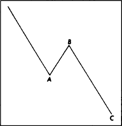
Figure 13.4 Bull Market Zig-Zag (5-3-5). (Frost and Prechter, p. 36. Copyright © 1978 by Frost and Prechter.)
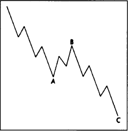
Figure 13.5 Bull Market Zig-Zag (5-3-5). (Frost and Prechter, p. 36. Copyright © 1978 by Frost and Prechter.)
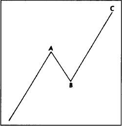
Figure 13.6 Bear Market Zig-Zag (5-3 5). (Frost and Prechter, p. 36. Copyright © 1978 by Frost and Prechter.)

Figure 13.7 Bear Market Zig-Zag (5-3-5). (Frost and Prechter, p. 36 Copyright © 1978 by Frost and Prechter.)

Figure 13.8 Double Zig-Zag. (Frost and Prechter, p. 37. Copyright © 1978 by Frost and Prechter.)
What distinguishes the flat correction from the zig-zag correction is that the flat follows a 3-3-5 pattern. Notice in Figures 13.10 and 13.12 that the A wave is a 3 instead of a 5. In general, the flat is more of a consolidation than a correction and is considered a sign of strength in a bull market. Figures 13.9-13.12 show examples of normal flats. In a bull market, for example, wave B rallies all the way to the top of wave A, showing greater market strength. The final wave C terminates at or just below the bottom of wave A in contrast to a zig-zag, which moves well under that point.
There are two “irregular” variations of the normal flat correction. Figures 13.13-13.16 show the first type of variation. Notice in the bull market example (Figures 13.13 and 13.14) that the top of wave B exceeds the top of A and that wave C violates the bottom of A.
Another variation occurs when wave B reaches the top of A, but wave C fails to reach the bottom of A. Naturally, this last pattern denotes greater market strength in a bull market. This variation is shown in Figures 13.17-13.20 for bull and bear markets.
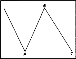
Figure 13.9 Bull Market Flat (3-3-5), Normal Correction. (Frost and Prechter, p. 38. Copyright © 1978 by Frost and Prechter.)

Figure 13.10 Bull Market Flat (3-3-5), Normal Correction. (Frost and Prechter, p. 38. Copyright © 1978 by Frost and Prechter.)
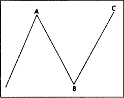
Figure 13.11 Bear Market Flat (3-3-5), Normal Correction. (Frost and Prechter, p. 38. Copyright © 1978 by Frost and Prechter.)

Figure 13.12 Bear Market Flat (3-3-5), Normal Correction. (Frost and Prechter, p. 38. Copyright © 1978 by Frost and Prechter.)
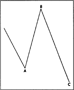
Figure 13.13 Bull Market Flat (3-3-5), Irregular Correction. (Frost and Prechter,p. 39. Copyright © 1978 by Frost and Prechter.)
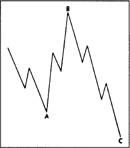
Figure 13.14 Bull Market Flat (3-3-5), Irregular Correction. (Frost and Prechter, p. 39. Copyright © 1918 by Frost and Prechter.)
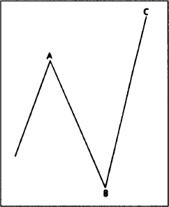
Figure 13.15 Bear Market Flat (3-3-5), Irregular Correction. (Frost and Prechter, p. 39. Copyright © 1978 by Frost and Prechter.)

Figure 13.16 Bear Market Flat (3-3-5), Irregular Correction. (Frost and Prechter, p. 39. Copyright © 1978 by Frost and Prechter.)

Figure 13.17 Bull Market Flat (3-3-5), Inverted Irregular Correction. (Frost and Prechter, p. 40. Copyright © 1978 by Frost and Prechter.)
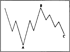
Figure 13.18 Bull Market flat (3-3-5), Inverted Irregular Correction. (Frost and Prechter, p. 40. Copyright © 1978 by Frost and Prechter.)

Figure 13.19 Bear Market Flat (3-3-5), Inverted Irregular Correction (Frost and Prechter, p. 40. Copyright © 1978 by Frost and Prechter.)
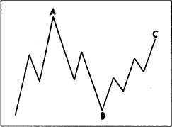
Figure 13.20 Bear Market Flat (3-3-5), Inverted Irregular Correction. (Frost and Prechter, p. 40. Copyright © 1978 by Frost and Prechter.)
Triangles usually occur in the fourth wave and precede the final move in the direction of the major trend. (They can also appear in the b wave of an a-b-c correction.) In an uptrend, therefore, it can be said that triangles are both bullish and bearish. They’re bullish in the sense that they indicate resumption of the uptrend. They’re bearish because they also indicate that after one more wave up, prices will probably peak. (See Figure 13.21.)
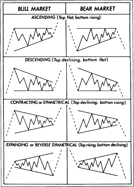
Figure 13.21 Corrective Wave (Horizontal) Triangles. (Frost and Prechter, p. 43. Copyright © 1978 by Frost and Prechter.)
Elliott’s interpretation of the triangle parallels the classical use of the pattern, but with his usual added precision. Remember from Chapter 6 that the triangle is usually a continuation pattern, which is exactly what Elliott said. Elliott’s triangle is a sideways consolidation pattern that breaks down into five waves, each wave in turn having three waves of its own. Elliott also classifies four different kinds of triangles—ascending, descending, symmetrical, and expanding—all of which were seen in Chapter 6. Figure 13.21 shows the four varieties in both uptrends and downtrends.
Because chart patterns in commodity futures contracts sometimes don’t form as fully as they do in the stock market, it is not unusual for triangles in the futures markets to have only three waves instead of five. (Remember, however, that the minimum requirement for a triangle is still four points—two upper and two lower—to allow the drawing of two converging trendlines.) Elliott Wave Theory also holds that the fifth and last wave within the triangle sometimes breaks its trendline, giving a false signal, before beginning its “thrust” in the original direction.
Elliott’s measurement for the fifth and final wave after completion of the triangle is essentially the same as in classical charting—that is, the market is expected to move the distance that matches the widest part of the triangle (its height). There is another point worth noting here concerning the timing of the final top or bottom. According to Prechter, the apex of the triangle (the point where the two converging trendlines meet) often marks the timing for the completion of the final fifth wave.
In its more general application, this rule or principle holds that the market usually doesn’t act the same way two times in a row. If a certain type of top or bottom occurred the last time around, it will probably not do so again this time. The rule of alternation doesn’t tell us exactly what will happen, but tells us what probably won’t. In its more specific application, it is most generally used to tell us what type of corrective pattern to expect. Corrective patterns tend to alternate. In other words, if corrective wave 2 was a simple a-b-c pattern, wave 4 will probably be a complex pattern, such as a triangle. Conversely, if wave 2 is complex, wave 4 will probably be simple. Figure 13.22 gives some examples.
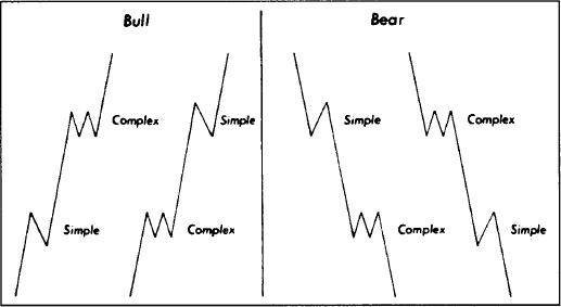
Figure 13.22 The Rule of Alternation. (Frost and Prechter, p. 50. Copyright © 1978 by Frost and Prechter.)
Another important aspect of wave theory is the use of price channels. You’ll recall that we covered trend channeling in Chapter 4. Elliott used price channels as a method of arriving at price objectives and also to help confirm the completion of wave counts. Once an uptrend has been established, an initial trend channel is constructed by drawing a basic up trendline along the bottoms of waves 1 and 2. A parallel channel line is then drawn over the top of wave 1 as shown in Figure 13.23. The entire uptrend will often stay within those two boundaries.
If wave 3 begins to accelerate to the point that it exceeds the upper channel line, the lines have to be redrawn along the top of wave 1 and the bottom of wave 2 as shown in Figure 13.23. The final channel is drawn under the two corrective waves—2 and 4—and usually above the top of wave 3 as shown in Figure 13.24. If wave 3 is unusually strong, or an extended wave, the upper line may have to be drawn over the top of wave 1. The fifth wave should come close to the upper channel line before terminating. For the drawing of channel lines on long term trends, it’s recommended that semilog charts be employed along with arithmetic charts.

Figure 13.23 Old and New Channels. (Frost and Prechter, p. 62. Copyright © 1978 by Frost and Prechter.)

Figure 13.24 Final Channel. (Frost and Prechter, p. 63. Copyright © 1978 by Frost and Prechter.)
In concluding our discussion of wave formations and guidelines, one important point remains to be mentioned, and that is the significance of wave 4 as a support area in subsequent bear markets. Once five up waves have been completed and a bear trend has begun, that bear market will usually not move below the previous fourth wave of one lesser degree; that is, the last fourth wave that was formed during the previous bull advance. There are exceptions to that rule, but usually the bottom of the fourth wave contains the bear market. This piece of information can prove very useful in arriving at a maximum downside price objective.
Elliott stated in Nature’s Law that the mathematical basis for his Wave Principle was a number sequence discovered by Leonardo Fibonacci in the thirteenth century. That number sequence has become identified with its discoverer and is commonly referred to as the Fibonacci numbers. The number sequence is 1, 1, 2, 3, 5, 8, 13, 21, 34, 55, 89, 144, and so on to infinity.
The sequence has a number of interesting properties, not the least of which is an almost constant relationship between the numbers.
It was already stated that wave theory is comprised of three aspects—wave form, ratio, and time. We’ve already discussed wave form, which is the most important of the three. Let’s talk now about the application of the Fibonacci ratios and retracements. These relationships can apply to both price and time, although the former is considered to be the more reliable. We’ll come back later to the aspect of time.
First of all, a glance back at Figures 13.1 and 13.3 shows that the basic wave form always breaks down into Fibonacci numbers. One complete cycle comprises eight waves, five up and three down—all Fibonacci numbers. Two further subdivisions will produce 34 and 144 waves—also Fibonacci numbers. The mathematical basis of the wave theory on the Fibonacci sequence, however, goes beyond just wave counting. There’s also the question of proportional relationships between the different waves. The following are among the most commonly used Fibonacci ratios:
The preceding ratios help to determine price objectives in both impulse and corrective waves. Another way to determine price objectives is by the use of percentage retracements. The most commonly used numbers in retracement analysis are 61.8% (usually rounded off to 62%), 38%, and 50%. Remember from Chapter 4 that markets usually retrace previous moves by certain predictable percentages—the best known ones being 33%, 50%, and 67%. The Fibonacci sequence refines those numbers a bit further. In a strong trend, a minimum retracement is usually around 38%. In a weaker trend, the maximum percentage retracement is usually 62%. (See Figures 13.25 and 13.26.)

Figure 13.25 The three horizontal lines show Fibonnaci retracement levels of 38%, 50%, and 62% measured from the 1981 bottom to the 1993 peak in Treasury Bonds. The 1994 correction in bond prices stopped right at the 38% retracement line.
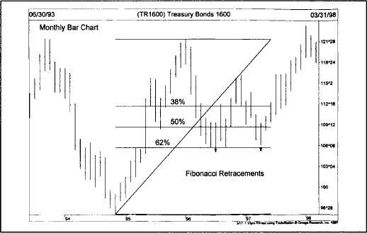
Figure 13.26 The three Fibonacci percentage lines are measured from the 1994 bottom in bond prices to the early 1996 top. Bond prices corrected to the 62% line.
It was pointed out earlier, that the Fibonacci ratios approach .618 only after the first four numbers. The first three ratios are 1/1 (100%), 1/2 (50%), and 2/3 (66%). Many students of Elliott may be unaware that the famous 50% retracement is actually a Fibonacci ratio, as is the two-thirds retracement. A complete retracement (100%) of a previous bull or bear market also should mark an important support or resistance area.
We haven’t said too much about the aspect of time in wave analysis. Fibonacci time relationships exist. It’s just that they’re harder to predict and are considered by some Elliotticians to be the least important of the three aspects of the theory. Fibonacci time targets are found by counting forward from significant tops and bottoms. On a daily chart, the analyst counts forward the number of trading days from an important turning point with the expectation that future tops or bottoms will occur on Fibonacci days—that is, on the 13th, 21st, 34th, 55th, or 89th trading day in the future. The same technique can be used on weekly, monthly, or even yearly charts. On the weekly chart, the analyst picks a significant top or bottom and looks for weekly time targets that fall on Fibonacci numbers. (See Figures 13.27 and 13.28.)
The ideal situation occurs when wave form, ratio analysis, and time targets come together. Suppose that a study of waves reveals that a fifth wave has been completed, that wave 5 has gone 1.618 times the distance from the bottom of wave 1 to the top of wave 3, and that the time from the beginning of the trend has been 13 weeks from a previous low and 34 weeks from a previous top. Suppose further that the fifth wave has lasted 21 days. Odds would be pretty good that an important top was near.

Figure 13.27 Fibonacci time targets measured in months from the 1981 bottom in Treasury Bonds. It may be coincidence, but the last four Fibonacci time targets (vertical bars) coincided with important turns in bond prices.
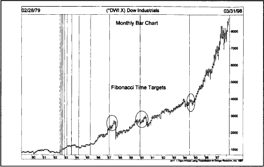
Figure 13.28 Fibonacci time targets in months from the 1982 bottom in the Dow. The last three vertical bars coincide with bear market years in stocks—1987, 1990, and 1994. The 1987 peak was 13 years from the 1982 bottom—a Fibonacci number.
A study of price charts in both stocks and futures markets reveals a number of Fibonacci time relationships. Part of the problem, however, is the variety of possible relationships. Fibonacci time targets can be taken from top to top, top to bottom, bottom to bottom, and bottom to top. These relationships can always be found after the fact. It’s not always clear which of the possible relationships are relevant to the current trend.
There are some differences in applying wave theory to stocks and commodities. For example, wave 3 tends to extend in stocks and wave 5 in commodities. The unbreakable rule that wave 4 can never overlap wave 1 in stocks is not as rigid in commodities. (Intraday penetrations can occur on futures charts.) Sometimes charts of the cash market in commodities give a clearer Elliott pattern than the futures market. The use of continuation charts in commodity futures markets also produces distortions that may affect long term Elliott patterns.
Possibly the most significant difference between the two areas is that major bull markets in commodities can be “contained,” meaning that bull market highs do not always exceed previous bull market highs. It is possible in commodity markets for a completed five wave bull trend to fall short of a previous bull market high. The major tops formed in many commodity markets in the 1980 to 1981 period failed to exceed major tops formed seven and eight years earlier. As a final comparison between the two areas, it appears that the best Elliott patterns in commodity markets arise from breakouts from long term extended bases.
It is important to keep in mind that wave theory was originally meant to be applied to the stock market averages. It doesn’t work as well in individual common stocks. It’s quite possible that it doesn’t work that well in some of the more thinly traded futures markets as well because mass psychology is one of the important foundations on which the theory rests. Gold, as an illustration, is an excellent vehicle for wave analysis because of its wide following.
Let’s briefly summarize the more important elements of wave theory and then try to put it into proper perspective.
The Elliott Wave Principle builds on the more classical approaches, such as Dow Theory and traditional chart patterns. Most of those price patterns can be explained as part of the Elliott Wave structure. It builds on the concept of “swing objectives” by using Fibonacci ratio projections and percentage retracements. The Elliott Wave Principle takes all of these factors into consideration, but goes beyond them by giving them more order and increased predictability.
There are times when Elliott pictures are clear and other times when they are not. Trying to force unclear market action into an Elliott format, and ignoring other technical tools in the process, is a misuse of the theory. The key is to view Elliott Wave Theory as a partial answer to the puzzle of market forecasting. Using it in conjunction with all of the other technical theories in this book will increase its value and improve your chances for success.
Two of the best sources of information on Elliott Wave Theory and the Fibonacci numbers are The Major Works of R.N. Elliott, (Prechter, Jr.) and the Elliott Wave Principle (Frost and Prechter). All of the diagrams used in Figures 13.1-13.24 are from the Elliott Wave Principle and are reproduced in this chapter through the courtesy of New Classics Library.
A primer booklet on the Fibonacci numbers, Understanding Fibonacci Numbers by Edward D. Dobson, is available from Traders Press (P.O. Box 6206, Greenville, S.C. 29606 (800-927-8222).