23

INFLATION AND RECENT
DEVELOPMENTS IN
COSMOLOGY

J. RICHARD GOTT

This chapter explores the very early universe—going back as far as the Big Bang and even before. As we have discussed, in 1948 George Gamow wondered what the universe would be like at its very earliest moments. Gamow reasoned that the universe would be compressed near the Big Bang and would be very hot and filled with hot thermal radiation. This radiation cools off as the universe expands.

We can explain this by thinking about the 3-sphere Friedmann universe. At each epoch, it has a finite circumference, and as this 3-sphere universe expands, its circumference increases. Imagine photons circling this circumference, like race cars going around a circular race track. The circumference of the track is getting bigger with time as the cars are continually chasing each other around the track. Suppose 12 photons are equally spaced around the circular track like the 12 numerals on a clock face. As the track expands, the cars are all racing at the same speed, the speed of light. If they start equally spaced around the track, with 1/12 of the track separating each car from the one in front of it, they will remain equally spaced around the track as it expands. Each car is equally good, so a car will not be catching up with the car in front or falling behind and running into the car behind. If the cars remain equally spaced around the track, as the circumference of the track gets larger, the distance separating the cars will increase. If the track doubles in size, the distances between the cars will double. Now imagine an electromagnetic wave circling the circumference going clockwise. Each of the 12 photons could be placed at one of the crests of the waves. The photons and the crests of the waves both travel at the speed of light, so the photons stay at the wave crests as the wave moves. Thus, as the track circumference expands, the distance between the wave crests expands by the same factor. When the circumference of the universe doubles, the wavelength (distance between the crests) doubles as well.

This explains why light will be redshifted as the universe expands: because of the stretching of space. This redshifting means that the hot thermal radiation in the early universe will cool off (become of longer wavelength) as the universe expands. Calculating the nuclear reactions occurring in the first 3 minutes and matching with the deuterium abundance we find today allowed Gamow’s students Robert Herman and Ralph Alpher to calculate the temperature that the radiation would have today by estimating how much the universe would have expanded since those early times. They got a current temperature of 5 K. In the 1960s, as we saw in chapter 15, Robert Dicke at Princeton thought of the same argument, came to similar conclusions, and decided to look for the radiation. Penzias and Wilson beat Dicke’s team to it.

When the Cosmic Background Explorer (COBE) satellite was launched in 1989 to measure the cosmic microwave background (CMB) in detail, it found a nearly perfect blackbody shape for its spectrum (just as Gamow would have predicted) with a temperature of 2.725 K. George Smoot and John Mather received the 2006 Nobel Prize in Physics for their work on COBE.

Gamow and Alpher’s prediction of the existence of the CMB and Alpher and Herman’s estimate of its temperature as 5 K together constitute one of the most remarkable predictions in the history of science to be subsequently verified. It was rather like predicting that a flying saucer 50 feet across would land on the White House Lawn and later having one 27 feet across actually show up! This is also an important vindication of the Copernican Principle, the idea that our location must not be special; with Hubble’s observations of isotropy, the Copernican Principle leads us directly to the homogeneous, isotropic, Friedmann Big Bang solutions of Einstein’s field equations, which Gamow and his colleagues used to predict the microwave background.

The resulting Friedmann Big Bang model has been incredibly successful, but some important questions remained. This universe has a beginning, a Big Bang, but what happened before the Big Bang? The standard answer (which we gave in chapter 22) has been that time, as well as space, was created in the Big Bang, so there was no time before the Big Bang. Still people wondered, why was the Big Bang so uniform? When we look out in different directions, the temperature of the CMB is uniform to one part in 100,000. How do these different regions “know” to be at the same temperature? When we look in one direction, we see out 13.8 billion light-years. But we are looking back in time to an epoch when the universe was only 380,000 years old. In the standard Big Bang model, that region should be influenced only by stuff no more than 380,000 light-years away from it. But if we look out 13.8 billion light-years in the opposite direction, 180° across the sky, we see another region that is at essentially the same temperature. In the standard Big Bang model, these two regions on opposite sides of the sky at an epoch 380,000 years after the Big Bang (when we are seeing them) are separated by a distance of 86 million light-years and have not had time to communicate with each other in the scant 380,000 years since their birth. Usually, if we see two regions at the same temperature, it is because they have had time to communicate with each other and reach thermal equilibrium. But in the standard Big Bang model, widely separated parts of the CMB observable in the sky have not had time to be in causal contact with each other. In the Friedmann model, different regions of the universe must have miraculously started out with a homogeneous expansion at the same temperature everywhere. How could it be so uniform?

But COBE also detected small fluctuations of one part in 100,000 from one region of the sky to another. If the universe had been perfectly uniform, no density enhancements would have been present to grow into galaxies and clusters of galaxies later. Our existence depends on the universe having small fluctuations initially, which can eventually grow by the action of gravity into the galaxies we observe today. The universe had to be almost perfectly uniform but not quite. It was a mystery. I am reminded of the old Depression Era saying: “If we had some bacon, we could have bacon and eggs for breakfast, if we had some eggs!” We needed to explain first the overall uniformity and then the small fluctuations.

In 1981, Alan Guth proposed a solution to this problem. His model proposed that the universe started with a short period of accelerated expansion he called inflation. In a spacetime diagram, this looks like a small trumpet bell pointing upward like a golf tee, to hold up the Friedmann football spacetime. It starts with a finite circumference near the mouthpiece of the trumpet but becomes dramatically larger as we move upward in time to the bell-like opening of the horn. The bottom tip of the Friedmann football is replaced by a little trumpet mouth with finite circumference at the bottom—perhaps as small as 3 × 10^–27 centimeters (figure 23.1). The trumpet epoch lasts a little longer than the Big Bang tip of the football would alone, and this extra time allows the different regions we see today enough time to get into causal contact. In the beginning, the circumference is so small that the different regions, benefiting from that little bit of extra time, come into casual contact, and then the accelerated expansion during the trumpet epoch pulls them far apart; it only looks as though they have had insufficient time to be in communication.

FIGURE 23.1. Inflationary beginning (trumpet) to start a Friedmann Big Bang universe (football).

Photo credit: J. Richard Gott

What was Guth’s basis for this model? He thought that in the early universe there may have been a vacuum state having a high energy density—and therefore a high negative pressure—mimicking the curvature of empty space implied by Einstein’s famous cosmological constant. But Guth wanted a very high value for this cosmological constant. We are used to thinking that empty space should have a zero density. It has, after all, been cleared of all particles and radiation. But the vacuum of empty space may have an energy density due to fields like the Higgs field filling the universe. The amount of vacuum energy present depends on the laws of physics. Guth argued that in the early universe, the weak and strong and electromagnetic forces would have been united in a single superforce, and the vacuum energy at that time (when the laws of physics were different) might have been much higher than the tiny value seen today. Thus the cosmological constant was not really a constant (as Einstein had supposed) but could change with time. In the very early universe, the vacuum energy density could have been quite high. Accompanying this high energy density was a large negative pressure, ensuring, by the laws of special relativity, that the vacuum energy as seen by different observers traveling at different velocities through space would all be the same. As we have discussed, the vacuum energy density produces an attraction, but the negative pressure operating in three directions produces a gravitational repulsion three times larger. This, according to Einstein’s equations, would have started the universe off on the accelerated expansion Guth wanted. It was this gravitational repulsion that produced the initial expansion we call the “Big Bang.”

In fact this trumpet-like solution to Einstein’s field equations had already been found by Willem de Sitter in 1917. He solved Einstein’s equations for the case of empty space with a cosmological constant and nothing else. With no ordinary matter to balance the repulsive effects of the cosmological constant, this solution produced a universe whose expansion was accelerated. The whole solution is called de Sitter space. This spacetime is a 3-sphere universe that starts off with infinite radius in the infinite past. It is contracting at nearly the speed of light. But the repulsive effects of the cosmological constant begin to slow the contraction until it stops at a minimum radius—a waist of minimum circumference—and then begins to expand. It expands faster and faster as the repulsive effects of the cosmological constant continue. It ends up expanding at a rate closer and closer to the speed of light, and in the infinite future this universe expands to infinite size. The spacetime diagram of de Sitter spacetime looks like a corset with a narrow waist (figure 23.2). The diagram shows one dimension of space around the horizontal circumference and the dimension of time vertically. The future is toward the top. The skirt at the bottom shows the contracting phase, and the waist at the middle shows the minimum radius of the universe. Then it fans out at the top to make a trumpet horn.

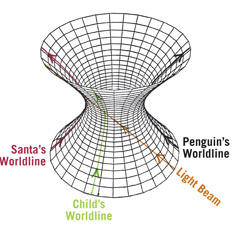
FIGURE 23.2. A spacetime diagram of de Sitter space. As in figures 22.4 and 22.5, this figure shows one dimension of space and one of time. Credit: J. Richard Gott

As with the Friedmann spacetime model, the only thing to pay attention to here is the corset-shaped surface itself. Forget the inside and outside. The surface alone is real. This corset-shaped spacetime has horizontal circular cross-sections at individual time slices. These show the circumference of the 3-sphere universe at particular instants of cosmic time. These circles are large at the bottom, reach a minimum at the waist, and then get larger again at the top, showing the size of the 3-sphere universe as it contracts and then expands. The vertical “corset stays” represent possible worldlines of particles. These are straight geodesic lines that little trucks could follow by traveling straight ahead on the corset’s surface. The corset stays are coming together in the bottom half, reach a minimum separation at the waist, before spreading apart in the upper half. In the upper half, the curvature of the spacetime is causing these particles to accelerate away from each other. As the particles fly apart, their clocks begin to slow down exponentially as they approach the speed of light. Their clocks are s_l__o___w___i____n_____g______d______o_______w________n. During later ticks on these clocks, the circumference expands enormously. Although the diagram shows the space to be expanding approximately linearly at nearly the speed of light at late times (a cone opening out at nearly 45°), as measured by the exponentially slowing clocks carried by the particles themselves, the circumference seems to be doubling in each successive time interval, increasing as 1, 2, 4, 8, 16, 32, 64, 128, 256, 512, 1,024, . . . , resulting in an exponentially accelerated expansion. It’s like currency inflation, which is why Guth called the model inflation.

Look at the waist. It is a circle representing the 3-sphere universe at its point of maximum contraction. Keep in mind that it is really a 3-sphere. We can designate the point on the far left of this circle as a “north pole” of this universe. Santa would live there. Consider the red corset stay at the left: it is the worldline of Santa sitting at the north pole of the 3-sphere universe. The corset stay at the right, 180° away, is the black worldline of a penguin at the south pole. Santa, whose worldline is at the north pole, will never see the penguin living at the south pole. A light beam starting from the penguin in the infinite past will travel straight at 45° upward and to the left. It will pass diagonally upward across the front of the corset like a diagonal sash, but it will never quite reach Santa’s worldline at the left. There are event horizons in this universe. Santa never sees anything that happens to the penguin—he never sees anything upward and to the right of that sash. Consider a child living near Santa, whose green worldline is shown in figure 23.2. Light beams from that child can reach Santa. Santa will see the child at late times accelerating away from him. Light from the child will become more and more redshifted. If the child sends Santa a message that says “THINGS ARE GOING FINE,” Santa will receive “THINGS A_R__E.” But Santa will never receive the signals “GOING FINE.” The signal “GOING” travels along that 45° sash and never arrives. It looks to Santa just as though the child were falling down a black hole. When the child’s worldline crosses that 45° sash, which is Santa’s event horizon, the child’s signals no longer arrive. The space between Santa and the child is simply stretching so fast that the signal “FINE,” emitted on the other side of the sash, cannot traverse the ever-widening distance between Santa and the child. This does not violate special relativity. The latter just says someone else’s spaceship cannot pass you at a speed faster than the speed of light. But general relativity still allows the space between two particles to stretch so fast that light cannot cover the ever-widening gap between them. De Sitter spacetime explains how particles can get into communication and thermal equilibrium near the waist and then be spread apart to great distances.

Guth was ultimately proposing to start the de Sitter universe at the waist, with a small circumference that today we might estimate to be perhaps as small as approximately 3 × 10^–27 centimeters. He was eliminating the infinite contraction phase (the lower half of the full spacetime). He just needed a little bit of high-density vacuum state at the beginning. The repulsive effects of the large negative pressure would cause the spacetime to start expanding, and then to expand faster and faster, with the size of the universe doubling every 10^–38 seconds. The universe would become very large. As the universe expanded, the energy density of the vacuum state would stay the same. The cosmological constant would stay constant. A small region of high energy density would expand to become a large region having the same high energy density.

Curiously, this would not violate local energy conservation. If I had a box of high-density, negative-pressure fluid, as I expanded the walls of the box, I would have to do work to pull the walls apart against the negative pressure that was resisting expansion. The work I was doing pulling the walls apart against this negative pressure (or suction) would add energy to the fluid—just enough to keep its energy density at the same high level as the volume of the box expanded. Thus energy would be conserved locally. But in the universe, what is pulling on the walls of my box? It is just the negative pressure from the other little similar boxes of spacetime next to it. As long as the pressure is uniform throughout the universe, the expansion itself is doing the work.

In general relativistic cosmology, there is no global energy conservation, because there is nowhere flat (approximating the spacetime of special relativity) on which to stand and establish an energy standard. Thus the total energy content of the universe can go up with time if there is negative pressure. This enabled Guth to start off his inflation model with a little piece of high-density vacuum and then let it grow naturally into a large universe with a vacuum state of the same density. In this way the vacuum state was “self-reproducing,” growing exponentially large from a tiny beginning. Because of this, Guth said the universe “is the ultimate free lunch.” Eventually, the vacuum state would decay, as the strong and weak and electromagnetic forces decoupled. As the energy density in the vacuum of empty space dropped to a low value, its vacuum energy would be dumped into the form of elementary particles. The universe would fill with a thermal distribution of elementary particles.

This is where the inflationary trumpet at the beginning of the universe joins to the bottom of the football-shaped Friedmann Big Bang model. The expansion of the universe then starts to decelerate, as in the football model. The pressure is now just the ordinary thermal pressure of particles, which is positive. Worldlines that have said “goodbye” to each other during the accelerating inflationary trumpet phase (like Santa and the child), will say “hello again” after the decelerating Friedmann phase begins. Inflation showed how the initial conditions of the Friedman Big Bang model could be naturally produced. The repulsive gravitational effects of the initial vacuum state (through its negative pressure) started the Big Bang! The Big Bang did not have to start with a singularity, but instead could start with a small, high-density vacuum region. Inflation could explain why the universe was so large, and why it was so uniform. Any wrinkles would be flattened out as the universe stretched to enormous size. It could also explain the small fluctuations of 1 part in 100,000 that we observe. These are small random quantum fluctuations due to Heisenberg’s uncertainty principle. The universe was doubling in size every 10^–38 seconds in the beginning; on these short timescales, the uncertainty principle ensures random fluctuations in the energy of any field. In fact, the spongelike pattern of galaxy clustering that we see in the universe today—the cosmic web, as well as the pattern of hot and cold spots in the CMB, indicate that the initial conditions appear to have been random in precisely the way expected from the random quantum fluctuations predicted by inflation (see my book, The Cosmic Web [2016]).

Inflation had one problem, however, which Guth recognized. The high-density vacuum state at the beginning would not be expected to decay into elementary particles all at once. This high-density inflating sea would decay into bubbles of low-density vacuum, a phenomenon investigated by Sidney Coleman. It is like boiling water in a pot. The water does not turn to steam all at once. Bubbles of steam form in the water. But this was not a uniform distribution—not the uniform universe we were hoping for. So Guth mentioned that as a problem. In 1982, I proposed that inflation would produce bubble universes—each bubble would expand to make a separate universe like ours (figure 23.3).

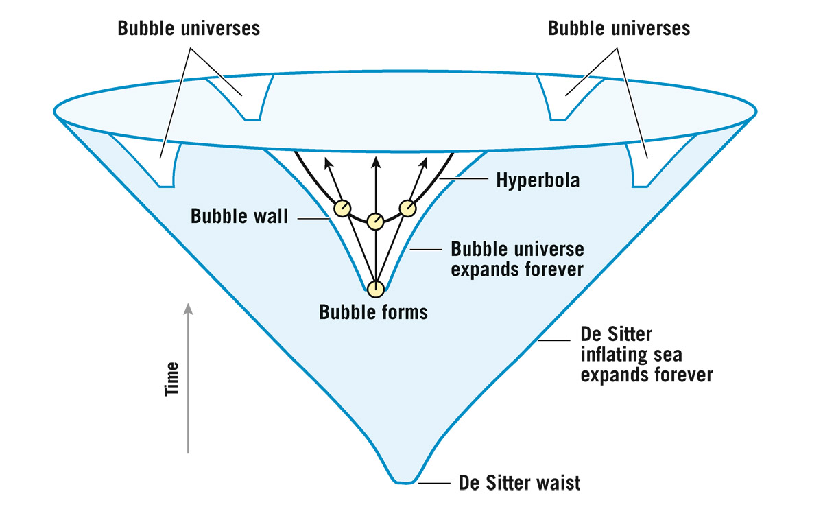
FIGURE 23.3. Bubble universes forming in an inflating sea—A multiverse.

Credit: Adapted from J. Richard Gott (Time Travel in Einstein’s Universe, Houghton Mifflin, 2001)

In my theoretical model, we live inside one of the low-density bubbles. I noticed that if, after the bubble formed, it took a while for the vacuum energy to decay, it would decay on a hyperbolic surface, making a uniform, negatively curved, hyperbolic Friedmann cosmology (recall figure 22.6). From inside the bubble, we are looking out in space and back in time, so we just see our own bubble universe and the uniform inflating sea before it was created. Everything looks uniform to us—solving Guth’s nonuniformity problem. The bubble expands at nearly the speed of light. But the inflating sea expands so fast that the bubbles never percolate to fill the entire space. New bubble universes are continually forming, and the inflating sea is expanding between them to provide space for even more new bubble universes to form. I envisioned an infinite number of bubble universes forming in an ever-expanding inflating sea—what we now call a multiverse.1 These bubble universes would have negative curvature inside and would expand forever—they would be hyperbolic Friedmann universes. Surfaces of constant epoch would be hyperbolas nestled inside the expanding bubble. A surface of constant epoch is one for which alarm clocks on individual particles all go off showing a constant time since the bubble formation event. Its shape is hyperbolic, because particles going faster have clocks that tick more slowly and therefore, the point at which their alarm clocks go off is delayed (compare with figure 22.6). This produces a hyperbolic shape that is infinite in extent as it bends upward inside the expanding bubble wall (see figure 23.3). Eventually, as the bubble expands to infinite volume in the infinite future, an infinite number of galaxies would be produced. Thus, an infinite number of infinite bubble universes could be produced from an initially very small, high-density de Sitter space.

This seems odd. How can one get an infinite number of universes each ultimately infinite in size, from just a finite beginning? De Sitter spacetime looks like a trumpet with its mouth opening upward. A horizontal slice through the waist of de Sitter space at the mouth of the trumpet is a circle. This is a small 3-sphere universe of finite circumference and finite volume, like the one Einstein considered. But the top of the trumpet resembles a cone, and one can slice a cone in a circle, a parabola, or a hyperbola, depending on how you slice it. If you slice de Sitter spacetime horizontally, you get a circle—that’s a 3-sphere universe. If you slice it on a 45° slant, you get a parabola and an infinite flat universe. If you slice it with a vertical plane, you will get a hyperbola—that makes an infinite negatively curved universe. It is like the old fable about the blind men and the elephant. One man feels the trunk and says the elephant is shaped like a snake. Another feels the leg and says that the elephant is shaped like a tree trunk. Still another feels the side of the elephant and says it is like a wall. In the same way, the shape of de Sitter space depends on how you slice it. Make one hyperbolic slice inside a bubble universe that extends to infinity, and you have a slice of space that is infinite, marking the epoch where the inflating de Sitter vacuum ends and dumps its energy into particles, and the Friedmann model begins. Just like a loaf of bread, which can be cut into different slices to make American slices or French slices, the real thing is the loaf itself. If we look at the spacetime geometry of de Sitter space for the inflationary model, we can see that it starts as a finite 3-sphere universe at the waist and expands forever, becoming infinitely large. This remarkable spacetime geometry, in which inflation continues forever and the space becomes infinitely big, allows creation of an infinite number of infinite bubble universes in an ever-inflating sea.

Different bubble universes could have different laws of physics in them, if different bubbles corresponded to tunneling and rolling down into different valleys in the landscape, where the values of various fields could be different. The laws of physics we see in our universe could be only local bylaws, as emphasized by Andrei Linde and Martin Rees.

It is important for the de Sitter inflationary universe to begin at the waist. We do not want the infinite contraction phase that precedes it. Borde and Vilenkin showed why: bubbles would form in the contracting phase too, and there the bubbles would be expanding in a space that was contracting; the low-density bubbles would collide with one another and fill up the space, ending the inflating sea and preventing it from ever reaching the waist and the expansion phase. You would just get a Big Crunch singularity; the bubbles would not have negative pressure inside to cause a turnaround at the waist. So, Borde and Vilenkin concluded that the inflationary multiverse starts off as a finite piece of inflating sea at the beginning. This could be small, as small as 3 × 10^–27 centimeters. It isn’t nothing, but it is perhaps as close to nothing as you could get.

The vacuum energy density can be viewed as the altitude in a landscape. The altitude represents the vacuum energy density, the energy density of empty space. Different places in the countryside correspond to different values of the fields (such as the Higgs field) that are creating the vacuum energy. Different locations (different values of the fields) correspond to different altitudes (different values of vacuum energy density). Today we have a very low vacuum-energy density—we are near sea level. But in the early universe the vacuum energy density would be high, like being trapped in a high mountain valley (figure 23.4).

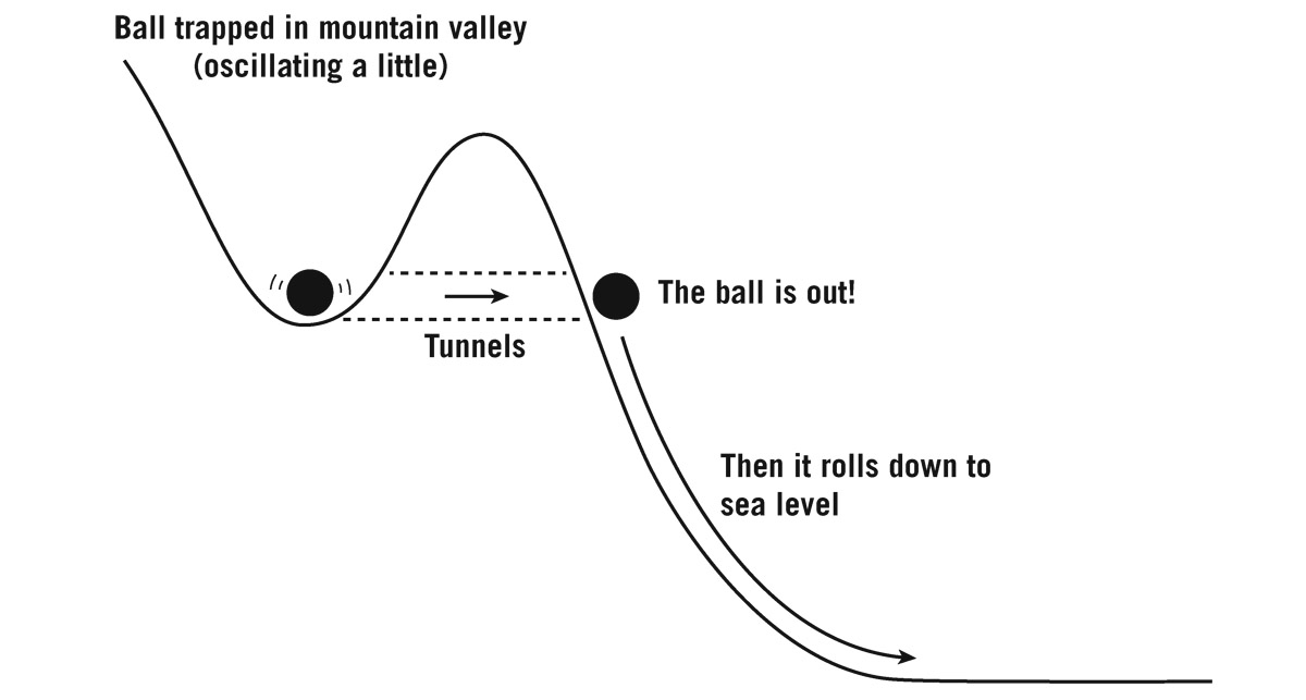
FIGURE 23.4. Quantum tunneling.

Credit: Adapted from J. Richard Gott (Time Travel in Einstein’s Universe, Houghton Mifflin, 2001)

A ball trapped in a high mountain valley is ultimately unstable: it has a lower energy state it can go to—sea level. But it can be trapped if it is surrounded by mountains on all sides. In Newton’s universe, it would have no way to roll down, but the quantum mechanical process called quantum tunneling allows it to tunnel through a surrounding mountain and then roll down to sea level.2

Quantum tunneling is a process discovered by George Gamow. It explained the radioactive decay of uranium. Uranium nuclei decay by emitting an alpha particle (a helium nucleus with two protons and two neutrons). The alpha particle is trapped inside the nucleus by the strong nuclear force attracting it to other protons and neutrons. This strong force acts like the mountain range surrounding the mountain valley, trapping the alpha particle inside the nucleus. But the strong nuclear force is a short-range force; if the alpha particle could somehow get out of the nucleus, beyond the influence of the strong-force attraction, it could escape. The alpha particle is positively charged and would then be repelled by the positively charged main nucleus. It would roll down the hill, away from the nucleus, and the kinetic energy it picked up would be due to electrostatic repulsion. From the energy an emitted alpha particle is measured to have when uranium decays, scientists could calculate how high up the hill it was when it began. It turned out that it was emitted outside the uranium nucleus! How did it get out there? Quantum mechanics tells us that just as light has both a wave and a particle nature, so too do objects we usually refer to as “particles,” such as alpha particles. The wave nature of an alpha particle means that it is not well localized, in a sense captured by Heisenberg’s uncertainty principle. Gamow found there was a small probability that the alpha particle could “tunnel” through the mountain that was holding it inside the uranium nucleus and find itself suddenly far outside the nucleus, where it would roll down the hill away from the nucleus due to electrostatic repulsion. It reminds me of the Zen koan: How does the duck get out of the bottle (whose neck is too narrow to allow the duck to escape)? Answer: The duck is out! So the alpha particle quantum tunnels through the mountain and “the alpha particle is out.” Here is another instance where Gamow might have gotten a Nobel prize.

In the bubble universe case, the mountain valley represents the initial inflationary universe (at the waist of de Sitter space) with its high vacuum energy density. It would be happy to stay in that high-density ever-expanding state forever, but after a long time, there is a chance it will tunnel through the mountain, where it will roll down to sea level, releasing the energy of the vacuum into kinetic energy and into the creation of ordinary elementary particles. This tunneling represents the instantaneous formation of a small bubble with a vacuum energy density slightly less than the vacuum energy density outside. The negative pressure outside the bubble is stronger than the negative pressure inside the bubble, and the difference pulls the bubble wall outward. It expands faster and faster, eventually approaching the speed of light. Meanwhile, inside the bubble, the vacuum energy density is slowly rolling down the hill toward sea level. Inflation continues for a while inside the bubble as it rolls down the hill. When it has rolled to sea level and deposited its vacuum energy in the form of particles, inflation stops, and the Friedmann phase begins. It was this type of scenario that Andrei Linde and also Andreas Albrecht and Paul Steinhardt independently published shortly after my paper came out. Outside the bubble, the vacuum state remains up in the mountain valley and an endless inflating sea continues its rapid accelerated expansion. I had discussed the geometry and general relativity involved in the formation of bubble universes to make what today we call a “multiverse,” while Linde and Albrecht and Steinhardt independently proposed detailed particle physics scenarios that would actually allow bubble universes to be formed. I required that inflation continue in the bubble universe for a while to create the universe we live in. In the Linde and Albrecht and Steinhardt models, this did naturally occur as the vacuum energy density in the bubble took some time to roll slowly down the hill toward sea level. Later in 1982, Stephen Hawking published a paper adopting the bubble universe idea and showing that initial quantum fluctuations would be expanded by inflation to appear on cosmological scales, having just the form needed to successfully seed the formation of galaxies and clusters of galaxies in the universe.3 The structure that was subsequently observed in both the CMB and the galaxy distribution, which we described in chapter 15, is in beautiful accord with predictions from inflation.

Although it is possible for a neighboring bubble universe to collide with ours in the far future (perhaps 10¹⁸⁰⁰ years from now, creating a sudden hot spot in the sky whose radiation would probably kill any life around at the time), most of these other universes in the multiverse are forever hidden from our view by an event horizon. They are so far away that the light from them can never cross the ever-inflating region between us and them. It seems clear today that once it gets started, inflation is hard to stop. It will continue expanding forever, creating a multiverse with an infinite number of universes like ours. In 1983, Linde proposed chaotic inflation, which would also produce a multiverse of low-density pocket universes in an ever-expanding inflating sea. Linde’s chaotic inflation model relied on quantum fluctuations to move you randomly on the landscape. There was a chance that a quantum fluctuation would move you up into the hills or mountains, where the vacuum energy density was high. The higher the altitude, the higher the energy density, and the shorter the doubling time for expansion. In the high-altitude regions, more space of high vacuum energy density is being created at a rapid rate by the high rate of inflation. Regions at high altitude thus reproduce more rapidly. It’s as if people had more children the higher altitude at which they lived. After a few generations, almost everyone would be living in the mountains. The whole multiverse would be inflating at a high rate. Then individual regions could roll down into the valley, creating individual pocket universes like ours. Most of the volume of space would be in the rapidly expanding mountain regions, but there would be patches (pocket universes) always forming by rolling down to sea level. So, we don’t really need to start in mountain valleys. In a general landscape, we expect always to be forming low-density universes like ours in an ever-inflating multiverse.

Even though we can’t see these other universes in the multiverse, we have reason to think they exist, because they seem to be an inevitable prediction of the theory of inflation, which explains a wealth of observational data.

Inflation got a great boost when the WMAP and the Planck satellite produced their results. The strength of the temperature fluctuations seen at different angular scales in the CMB matches exactly the pattern expected from inflation (recall figure 15.3). The WMAP and Planck satellite observations also showed that the universe has approximately zero curvature. In a positive curvature universe, we would see fewer spots in the microwave background map, because the circumference of a large circle is smaller than the 2πr that we expect from Euclidean geometry. If it were negatively curved, the circumference would be larger than 2πr, there would be more spots, and the spots would be smaller in angular size than expected from Euclidean geometry. The observations show temperature fluctuations that peak in strength at about 1° in angular scale. This agrees with the prediction of a zero curvature universe.

This means that we don’t really know sign of the curvature. The curvature of the universe is just so low that we cannot measure it. Our current data show that the visible universe is flat to an accuracy of somewhat better than 1%. In the same way, a basketball court looks flat even though we know it follows the curvature of Earth. It’s just that the radius of Earth is very much larger than the basketball court, ensuring that the curvature in the basketball court is not noticeable. We know that early people thought Earth was flat, because the tiny part of Earth they could see was approximately flat. All we really know is that the radius of curvature of the universe is much larger than the 13.8-billion-light-year radius out to which we can see—out to the CMB. Guth emphasized that no matter what shape the universe was initially (whether positively or negatively curved), inflation in the simplest models would usually yield enough expansion to make the universe much larger than the part we can inspect. Guth predicted that we would find an approximately flat universe, and he was right. If our universe is a bubble universe, it simply means that it continued to inflate for a long time inside the bubble, as the vacuum state was rolling down the hill after tunneling. A “long” period of inflation, say 1,000 doublings in size as seen from inside the bubble, could be accomplished in just 10^–35 seconds, if the doubling time was 10^–38 seconds. That would make the current radius of curvature of the universe 10²⁷⁴ times larger than the part we can see, so it would look flat.

Cosmological models today are defined by two parameters: Ω_m and Ω_Λ. The values of these parameters determine the expansion history of the universe, and whether it is finite (like a 3-sphere) or infinite in extent. The first parameter describes matter density and is given by Ω_m = 8πGρ_m/3H₀², where G is Newton’s gravitational constant, ρ_m is the average density of matter in the universe today (including both ordinary matter and dark matter), and H₀ is the Hubble constant today, quantifying how fast the universe is expanding. The numerator (8πGρ_m) describes the density in the universe (the amount of gravitational attraction), while the denominator of the fraction (3H₀²) describes the kinetic energy in the expansion. In simple Friedmann models where matter only is involved, Ω_m tells us whether the universe will expand forever or not: if Ω_m > 1, the gravitational attraction overcomes the kinetic energy of expansion and the universe ultimately collapses: this is the 3-sphere Friedmann football-shaped spacetime illustrated in figure 22.5. If Ω_m < 1, the kinetic energy of expansion overcomes the gravitational attraction, and we get the negatively curved Friedmann universe that expands forever. If Ω_m = 1, the kinetic energy balances the gravitational attraction and the model is flat; it expands slower and slower forever as the density goes down and the kinetic energy of expansion lessens with time. These Friedmann models all have Ω_Λ = 0, where there is no vacuum energy density in empty space—they lie along the bottom edge of figure 23.5.

If there is vacuum energy present today, we must also consider the value of the second parameter, which characterizes the vacuum energy density and is given by Ω_Λ = 8πGρ_vac/3H₀², where ρ_vac is the vacuum energy density (the energy density of dark energy) in the universe today. We use the subscript Λ to remind us that dark energy behaves like Einstein’s cosmological constant term Λ. We can display all possible cosmological models on a plane. The horizontal coordinate indicates the value of Ω_m (matter density), while the vertical coordinate represents Ω_Λ (vacuum energy−dark energy). A particular cosmological model is represented by a point in the plane in figure 23.5 with horizontal and vertical coordinates (Ω_m, Ω_Λ), representing a particular combination of values of matter density and dark energy density today.

If Ω_Λ is not zero we get models that fill the diagram. The red diagonal line shows the set of models with Ω₀ = Ω_m + Ω_Λ = 1, indicating they are flat, as inflation predicts. Models to the left of that red line are saddle shaped and infinite in extent, models to the right of the red line are 3-sphere universes. The black dotted necktie-shaped region shows the models consistent with data on the CMB from the Boomerang high-altitude-balloon telescope project in Antarctica, a key early experiment. It runs directly along the red line, showing that the CMB data favor the flat model. We can get another constraint on the cosmological model by directly measuring the expansion history of the universe from observations of the relationship between redshift and distance to distant objects. Scientists use so-called Type Ia supernovae, which are good standard candles; the area in the (Ω_m, Ω_Λ) plane allowed by the supernovae Ia observations is shown in light green. These data show the expansion of the universe is accelerated, and for this discovery, Saul Perlmutter, Brian Schmidt, and Adam Riess shared the 2011 Nobel Prize in Physics. Models with Ω_Λ > Ω_m/2 have an expansion that is accelerating today, the gravitational repulsion of the dark energy being greater than the gravitational attraction of the matter. The green area from the supernova data satisfies this inequality and indicates acceleration today. (Models with Ω_Λ < Ω_m/2 would have been decelerating today.) The black necktie region intersects the green region in a small overlap region around Ω_m ≈ 0.30 and Ω_Λ ≈ 0.70. These values are consistent with both the CMB data and the supernova data.

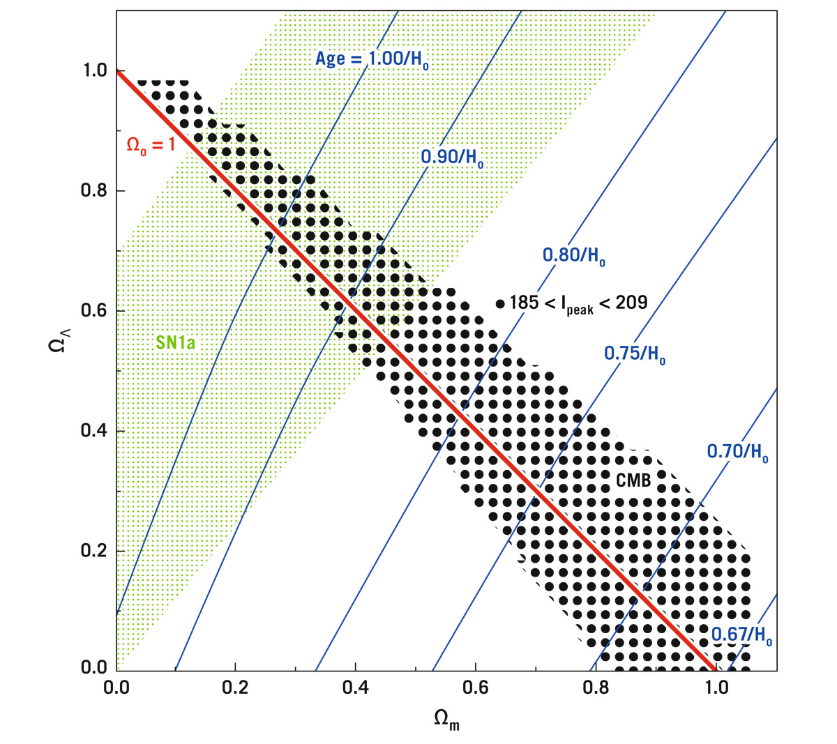
FIGURE 23.5. Cosmological models (Ω_m, Ω_Λ). Each point in this diagram represents a particular cosmological model with a particular value of matter density (corresponding to its horizontal coordinate Ω_m), and dark energy density (corresponding to its vertical coordinate Ω_Λ). The green dotted area covers models allowed by Supernova Ia observations (SN1a) showing the expansion of the universe is accelerating. The black dotted area covers models allowed by the cosmic microwave background (CMB) from the Boomerang Balloon Project in the year 2000, one of the first papers showing CMB plus supernovae observations imply a flat universe (Ω₀ = Ω_m + Ω_Λ = 1), with Ω_m ≈ 0.3 and Ω_Λ ≈ 0.7. Dark energy is 70% of the stuff of the universe. Subsequent observations from the WMAP and Planck satellites have greatly strengthened this conclusion.

Credit: Reprinted by permission from MacMillan Publishers Ltd: Nature, 404, P. de Bernardis, et al. April 27, 2000

Interestingly, this overlap region agrees with the value of Ω_m ≈ 0.30 from dynamical arguments based on the masses of clusters of galaxies, individual motions of galaxies, and the growth of structure in the universe. This includes both ordinary matter (baryons—protons and neutrons) and dark matter. Knowing the Hubble constant is approximately 67 (km/sec)/Mpc, it turns out that we can determine Ω_m and Ω_baryon directly by measuring the relative heights of the even and odd peaks in figure 15.3. The answer is Ω_baryon ≈ 0.05 and Ω_m ≈ 0.30. This result from the CMB agrees with the answer Ω_baryon ≈ 0.05 from Gamow-type nucleosynthesis arguments discussed in chapter 15 and tells us that most of the matter in the universe is in the form of dark matter (Ω_darkmatter ≈ 0.25), which cannot be made of ordinary matter (baryons). The search is on to discover the detailed nature of the dark matter, as Michael has described.

The blue lines in figure 23.5 show the age of the universe in terms of 1/H₀. The favored cosmological model is near the line marked “age = 1/H₀.”

Since the Boomerang results in 2000, the WMAP satellite has measured the CMB with high precision and refined these estimates to produce a standard cosmological model that explains all the observational constraints. The Planck satellite has further refined these estimates: H₀ = 67 (km/sec)/Mpc; age of the universe = 13.8 billion years; and a value of Ω_m + Ω_Λ = 1 within the observational errors, to an accuracy of better than 1%, consistent therefore with a flat model.

WMAP’s results, when combined with supernova and other data, were even able to track the expansion history of the universe, and through application of Einstein’s equations establish the ratio of the pressure to the energy density in the dark energy, a key measure that is simply called w. The value WMAP found for w = –1.073 ± 0.09, which is equal to the value of –1 predicted by Einstein’s cosmological constant model to within the observational errors. The Planck satellite produced a similar estimate. Recently, the Sloan Digital Sky Survey has measured the current value of w to be w₀ = –0.95 ± 0.07, using data on galaxy clustering and a fitting formula developed by Zack Slepian and myself. Using the same data and formula, but adding data from the magnitude of gravitational lensing of background by foreground galaxies, the Planck satellite team has found w₀ = –1.008 ± 0.068. All these estimates are consistent, within the observational errors, with the value of w = –1 expected from vacuum energy (dark energy). We know the energy density of dark energy is positive, because positive energy density, above and beyond that of ordinary matter and dark matter, is required to make the universe flat (which we observe). We know that the pressure of dark energy is negative, because, given that the energy density of dark energy must be positive, only a negative pressure for the dark energy could produce the gravitational repulsion required to cause the accelerating expansion of the universe that we observe. We can even accurately measure the amount of this negative pressure and find that it is equal to –1 times the energy density of the dark energy to within the observational errors. Einstein would be happy! His cosmological constant term was not a blunder after all!

Sometimes people say that dark energy is a mysterious force that is causing the current acceleration of the expansion of the universe, or that we know nothing about dark energy. That’s not really true. The force that is causing the accelerated expansion of the universe is just gravity. And it’s repulsive because of the negative pressure associated with dark energy. We strongly suspect that dark energy appears on the right side of Einstein’s equations with the stuff of the universe, rather than appearing on the left side of the equations as part of the law of gravity, because we suspect that a different (higher) amount of dark energy was present in the early universe, producing inflation. We suspect that dark energy is a form of vacuum energy produced by a field or fields, but we don’t know which one or ones. We know that the amount of dark energy is approximately constant with time, but we don’t know whether it is slowly falling (rolling down the hill) or rising (rolling up the hill). This is the focus of current research.

The Sloan Digital Sky Survey was able to make an accurate estimate of the Hubble constant, using a characteristic scale found in galaxy clustering corresponding to the oscillations seen in the fluctuations in the CMB in figure 15.3. In this way, they could replace the Cepheid variable ruler for establishing the overall scale, while using supernova data to chart the detailed changes in the Hubble constant with time. They found a value of H₀ = 67.3 ± 1.1 (km/sec)/Mpc. This means that the density of dark energy is about 6.9 × 10^–30 grams per cubic centimeter. If we were to draw a sphere centered on us with a radius equal to that of the Moon’s orbit, the mass equivalent of the amount of dark energy contained within this sphere would be 1.6 kilograms—inconsequential relative to the mass of Earth−which is so small that we don’t notice its slight gravitational effect or the slight gravitationally repulsive effect of its negative pressure on the orbit of the Moon. But its effects on cosmological scales, where the average density of matter is only 3 × 10^–30 grams per cubic centimeter, is profound.

Establishing this cosmological model with small errors is quite an accomplishment. The WMAP and Planck satellites have produced detailed measurements of the power of fluctuations as a function of angular scale in the CMB, which agree in extraordinary detail with the results predicted from inflation (as shown in figure 15.3). This is a dramatic experimental vindication of inflation. And the dark energy we see today is of exactly the form required for inflation in the early universe, but just of very low density.

A new independent test for inflation has recently been proposed. If inflation causes the universe to double in size approximately once every 10^–38 seconds, early on one could only see out to a distance of 10^–38 light-seconds or 3 × 10^–28 centimeters. This distance is tiny, and due to Heisenberg’s uncertainty principle of quantum mechanics, this causes fluctuations in the geometry of spacetime (ripples), which according to Einstein’s equations propagate at the speed of light—namely, gravitational waves. These would leave a characteristic swirling pattern in the polarization of the microwave background radiation which can be measured in principle. So far, its detection has proved elusive. The current best upper limits from the Planck satellite, plus ground-based experiments called Keck and BICEP2, lie somewhat below those of the simplest Linde chaotic inflation model. The amplitude of the gravitational waves produced depends on the detailed shape of the hill you are rolling down (see figure 23.4). The inflationary model the Planck team thinks fits the data best is one by Alexei Starobinsky; its doubling time is 3 × 10^–38 seconds at the end of the inflationary epoch, compared with the 5 × 10^–39 seconds doubling time in the simplest Linde model. This six-times-less-violent expansion would produce gravitational waves of six times lower amplitude, safely below the current upper limits. A number of observational efforts, including high-altitude balloons and ground experiments in Antarctica, are underway to lower the observational errors and further test inflationary models. Astronomers are anxiously waiting to see whether these observations can open a new window on the early universe.

With respect to the current universe, among the early astronomers working on cosmology in the twentieth century, the one who came closest to the truth was Georges Lemaître. In 1931, he proposed a model in which the universe started with a Big Bang and expanded like a Friedmann model, until it entered a coasting phase, during which the cosmological constant almost exactly balanced the matter density, approximating an Einstein static model for a while, after which time it expanded further, and the cosmological constant began to dominate as the matter thinned out. The spacetime diagram of this model looks like the lower half of a football at the bottom (Friedmann phase), then a cylinder (the Einstein static phase), and finally, the flared opening of a trumpet (de Sitter-space phase). Except for the coasting phase in the middle, Lemaître got it right. Lemaître was the first to calculate an expansion rate for the universe by combining Hubble’s distances to galaxies with Slipher’s redshifts. He was also the first to suggest that Einstein’s cosmological constant could be viewed as a vacuum state having positive energy density and negative pressure. Pretty good for one career!

Inflation has been very successful at explaining the structure of the universe that we see. We don’t really know how inflation got started, because inflation “forgets” its initial conditions as the universe exponentially expands, thinning out any initial components. But there are some speculations as to how inflation may have started.

Inflation can start with just a tiny de Sitter 3-sphere “waist” universe with a circumference of perhaps only 3 × 10^–27 cm, which will then start expanding. But where did that come from? Alex Vilenkin thought it might originate via quantum tunneling, a process analogous to that occurring with the formation of bubble universes. This time, the ball at rest in the mountain valley would correspond to a 3-sphere universe of zero size. It would then tunnel through the mountain to find itself suddenly outside on the slope. This would correspond to a finite-sized 3-sphere universe—the de Sitter waist. Then as it rolled down the hill, that phase would correspond to the de Sitter funnel. What would the spacetime diagram of this universe look like?

Vilenkin showed it would look rather like a badminton shuttlecock (figure 23.6). The point at the bottom is the pointlike zero-sized universe at the beginning. The feathered, funnel-shaped top of the shuttlecock is the de Sitter expansion at the end. Connecting the point at the bottom to the flaring funnel at the top is a black hemispherical ball shape. This represents the geometry during the tunneling through the mountain. Being “underground” in the tunnel causes the minus sign in front of the time dimension to flip sign: time becomes just another spacelike dimension. The hemisphere is half of a 4-sphere with four dimensions of space and no dimension of time. No clocks tick in this region: the tunneling occurs in a single instant. The ball is in the mountain valley and then suddenly it’s out. James Hartle and Stephen Hawking considered a model like this and added the idea that in this hemispherical bottom, the point at the beginning—the south pole—was no different from other points on the surface. It was exactly like the South Pole on Earth, which is likewise no different from other points on Earth’s surface. This universe has no boundary at the bottom—what Hawking calls the no boundary condition. Hawking has spoken of this early region as having imaginary time. The imaginary number i is the square root of –1. Normally, ds² = –dt² + dx² + dy² +dz², so if we had imaginary time, it, because i² = –1, the quantity –d(it)² would become +dt², and we would have ds² = dt² + dx² + dy² +dz². Imaginary time sounds spooky, but it just makes time into another ordinary dimension of space. We would have four dimensions of space in this region instead of three dimensions of space and one dimension of time.

FIGURE 23.6. The spacetime diagram of a universe that has tunneled from nothing.

Credit: J. Richard Gott (Time Travel in Einstein’s Universe, Houghton Mifflin, 2001).

Quantum tunneling is certainly weird. We are looking for something weird to happen at the beginning of the universe, because what happened then was truly remarkable. Maybe it could have been quantum tunneling. But you don’t really start with nothing. You start with a quantum state corresponding to a universe of size zero that knows all about the laws of physics and quantum mechanics. How does nothing know about the laws of physics? The laws of physics are simply the rules by which stuff behaves; if you have no stuff, what do the laws of physics mean? This is one of the problems with trying to make a universe out of nothing.

Meanwhile, Andrei Linde had noted that an inflating universe can give birth to another inflating universe via a quantum fluctuation. A de Sitter inflating trumpet horn could give birth to another inflating trumpet horn, which would sprout and grow off it, like a branch grows off a tree. In fact, this branch will inflate and grow to be as large as the trunk and sprout branches of its own. Branches will continue forming branches, making an infinite fractal tree of universes, all from one original trunk. Each individual branch is a funnel that could form bubble universes (as in figure 23.3). We would be living in a bubble universe in one of the branches, but still, you might ask yourself: where did the trunk come from?

Li-Xin Li and I tried to answer this question. We proposed that one of the branches curled back in time and grew up to be the trunk. Our model is illustrated in figure 23.7. Along the top, we see four funnel-shaped de Sitter inflating universes labeled 1, 2, 3, and 4, from left to right. Universe 2 gives birth to Universe 1. Universe 2 gives birth to Universe 3. Universe 3 gives birth to Universe 4. Universe 4 is the granddaughter universe of Universe 2. These branches will continue to expand and give birth to additional branches ad infinitum. These funnels do not hit one another—imagine them missing each other in some higher dimensional space. In this spacetime diagram, as in previous diagrams, only the surface itself is real.

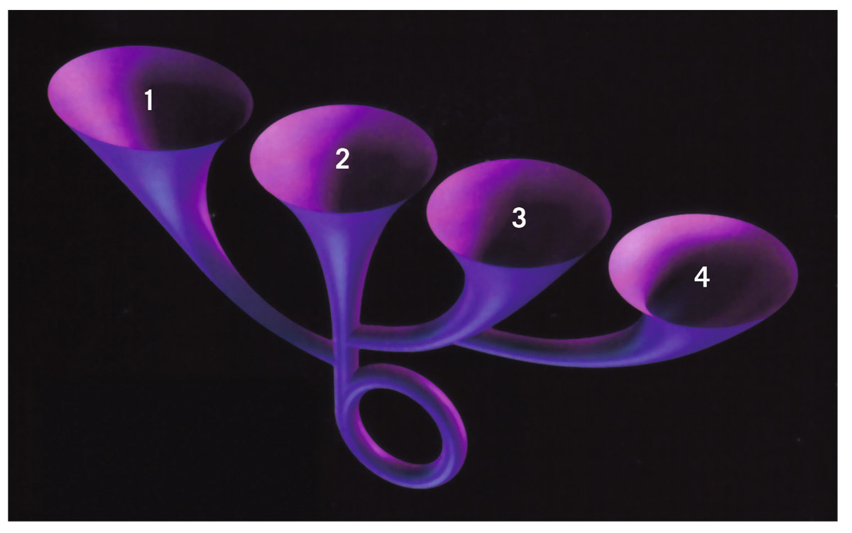
FIGURE 23.7. Gott–Li self-creating multiverse. The loop at the bottom represents a time machine; the universe gives birth to itself. Photo credit: J. Richard Gott, Robert J. Vanderbei (Sizing Up the Universe, National Geographic, 2011).

Now we come to the most surprising feature of the model: Universe 2 also gives birth to another branch that curls back in time and grows up to become the trunk. It creates a little time loop in the beginning that looks like the loop in the number “6.” Universe 2 is its own mother! As we have discussed, general relativity allows for loops in spacetime. There are no curvature singularities in this model. We were able to find a quantum vacuum state for this universe that was self-consistent and stable. The time loop has a Cauchy horizon marking the boundary where the time travel ends. It cuts at 45° across the trunk just above where the branch leaves the tree. You can continue to circle the loop in the “6” at the bottom as many times as you want, but when you move out beyond the branch into the top of the “6,” there is no going back. If you are before the Cauchy horizon, you can go back out the branch and back in time for another loop to visit yourself in the past, but once you cross the Cauchy horizon, you are beyond the branching point, and you just keep going on upward into one of the funnels at the top. This universe has a little time machine at the beginning that shuts down. Curiously, exiting such a time machine is stable, which actually makes building one at the beginning of the universe easier.

That’s interesting, because locating the time machine at the beginning of the universe puts it just where you want it to explain the first-cause problem. Every event in this universe has events that precede it. If you are anywhere in the time loop, there are always events counterclockwise from you that are before you and give rise to you in the usual causal way. This multiverse is finite to the past but has no earliest event. This can occur in a curved spacetime of general relativity.

This theoretical model would also seem to fit in well with superstring theory. Superstring theory or M-theory posits an eleven-dimensional spacetime consisting of one macroscopic dimension of time, three macroscopic dimensions of space, and seven additional spatial dimensions, which are curled up and microscopic, as Kaluza and Klein would have liked. The complex microscopic shape determines the laws of physics. Interestingly, inflation suggests that the three macroscopic spatial dimensions we see today were originally roughly as small as the microscopic Kaluza–Klein dimensions: a de Sitter waist of perhaps 3 × 10^–27 cm. This microscopic de Sitter circumference has inflated greatly as the universe has expanded. Originally, there were ten curled-up, microscopic spatial dimensions; seven have remained curled-up and tiny, while three have simply ballooned up in size since the beginning. Our (Gott–Li) model proposes that originally time was also curled up in a microscopic time loop. The time loop may have had a circumference in time (clockwise around the loop) as short as anywhere from 5 × 10^–44 to 10^–37 seconds if it had the self-consistent quantum vacuum state we have proposed. In the time loop, all ten dimensions of space as well as the dimension of time are curled up and tiny.

One of the wonderful things about inflation is that a small piece of inflating vacuum state expands to create a large volume, each little piece of which looks exactly like the piece you started with. If one of those little pieces is the piece you started with, then you have a time loop. Therefore, in our theory, the universe isn’t created from nothing but rather it is created from something, from a little piece of itself. Then the universe can be its own mother. Time travel is something unusual that appears to be allowed by general relativity; perhaps it is just what we need to explain how the universe got started.

Today, I would say the theory of inflation is in very good shape. It explains the fluctuations we see in the CMB in detail (recall figure 15.3). If you doubt that inflation occurred, remember that we see a low-grade inflation going on today. The universe’s expansion is accelerating, caused most likely by a low-density vacuum state (dark energy) with a density of 6.9 × 10^–30 grams per cubic centimeter. Inflation just relies on a large amount of dark energy in the early universe. Inflation seems inevitably to produce a multiverse of universes. Just how sure are scientists of this? Once Sir Martin Rees (the Astronomer Royal) was asked at a conference how sure he was that we lived in a multiverse. He said he wouldn’t be willing to bet his life on it, but he would go so far as to bet the life of his dog. Linde rose to say that since he had spent decades of his life working on the multiverse idea, he had proven that he would bet his life on it. Nobel Laureate Steven Weinberg said he would be willing to bet Linde’s life on it, and Martin Rees’s dog’s!

How did inflation begin? We don’t know. Did it emerge by quantum tunneling from nothing (perhaps the most popular model), or even stranger, was there a little time loop at the beginning? Pedro González-Díaz has speculated that when we have a true theory of quantum gravity, those two models might even turn out to be the same. Another speculation by Paul Steinhardt and Neil Turok is that the Big Bang occurred when two universes floating in an eleven-dimensional spacetime collided, heating them up suddenly. Repeated bangs could occur. (This would be rather like two pieces of paper—representing flatland universes—slapping together repeatedly in three-dimensional space. Such things could happen in principle in M-theory.) Lee Smolin thinks our universe could have been born inside a black hole in a previous universe. As a star collapsed to form a black hole, its interior density grew and grew until a high-density vacuum state was created, whose gravitationally repulsive nature caused it to bounce at a de Sitter waist and produce an expanding inflationary state that could spawn a multiverse, as pointed out by Claude Barrabès and Valeri Frolov. All this would occur inside the black hole that formed, the smile singularity in the Kruskal diagram being replaced by the start of a de Sitter expanding phase.

These are some of the speculative ideas that physicists are exploring to answer the ultimate question: how did the universe begin? Of these alternatives, probably the tunneling from nothing model is the most popular at the moment, but we simply don’t know which is correct. We may learn the answer when we find a “theory of everything,” which will unite general relativity and quantum mechanics and the strong, weak, and electromagnetic forces to explain all the laws of physics. When we have the equations of the “theory of everything,” we will see what cosmological solutions they produce. This is why we are studying fundamental physics. We are looking for clues about how the universe works, and maybe even how it began.