Catching Waves with an Oscilloscope

IN THIS CHAPTER

check Learning what an oscilloscope is

check Getting started with an oscilloscope

check Calibrating your scope

check Looking at waveforms

Electronics can generate some gnarly waves, dude. You’ll encounter all kinds of totally hairy waves in your electronic circuits. You meet sine waves, which just roll along nice and easy, like corduroy on the horizon. Sawtooth waves are epic: They ride up slow, then drop you way fast. And of course, square waves. They’re just, you know, square.

Your basic multimeter, which you learn about in the preceding chapter, is essential. You can’t do electronics without one. In this chapter, I tell you about another incredibly useful tool, called an oscilloscope. Although a voltmeter can give you a simple number that represents voltage, an oscilloscope can draw a picture of voltage. And, as they say, a picture is worth a thousand words — er, numbers.

Why is a picture so much more valuable than a number, when it comes to voltage? Because in all but the simplest circuits, voltage is always in motion; it’s always changing, and an oscilloscope is the perfect tool for observing voltage in motion.

As I said, an oscilloscope is an incredibly useful tool to have on your workbench. Although an oscilloscope is a bit expensive, you can pick up a good digital scope for under $100. You can get by for a while without an oscilloscope, but eventually you’ll want to get one.

The purpose of this chapter is really twofold. First, I want to show you how to use an oscilloscope should you manage to get your hands on one. Second, and perhaps more importantly, I want to convince you to start saving your pocket change so that someday you’ll be able to afford one. Once you get an oscilloscope on your workbench, you’ll wonder how you ever managed without it.

Understanding Oscilloscopes

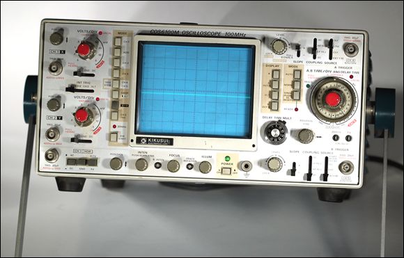
Figure 9-1 shows a typical oscilloscope. This one is an older model, but although oscilloscope technology has changed over the years, even older oscilloscopes are useful for basic circuit testing. If you invest in an oscilloscope, you’ll have a tool that will last you many, many years.

The most obvious feature of any oscilloscope is its screen. On older oscilloscopes, the screen is a cathode-ray tube (CRT) similar to an older television or computer monitor. On newer oscilloscopes, the screen is an LCD display like a flat-screen computer monitor.

Whether CRT or LCD, the purpose of the screen is the same: to display a simple graph of an electric signal. This graph, called a trace, shows how voltage changes over time. The horizontal axis of this graph, reading from left to right, represents time. The vertical axis, going up and down, represents voltage.

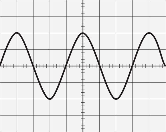
Figure 9-2 shows a typical oscilloscope display showing a very common type of trace known as a sine wave. Before I tell you about the sine wave, though, there are a few things to notice about the display:

Gridlines are printed on the display. On most oscilloscopes, these lines are 1 cm apart, with ten horizontal and eight vertical divisions.
The vertical and horizontal lines in the middle are thicker than the other lines and include hash marks, usually 2 mm apart. These hash marks help you pinpoint the exact position of the trace between the major intervals.
Various knobs and dials on the oscilloscope let you set the scale at which the graph of the waveform is plotted.
The vertical divisions represent voltage. On most oscilloscopes, you can set the voltage scale to as little as 5 mV (millivolts) and as much as 10 V or more. The oscilloscope usually represents 0 V by the horizontal line in the middle — so lines in the top half of the display represent positive voltage, and lines in the bottom half are negative voltage. Thus, if the voltage scale is set to 1 V, the display can show voltages between and . If you set the scale to 2 V, the display can show voltages between and .
The horizontal divisions represent time. The maximum time per division is typically 0.2 s (seconds), and the minimum time is typically – that’s half a microsecond. There are a million microseconds in a single second.

To draw a waveform, the oscilloscope actually draws a single dot that moves across the screen from left to right. Each passage of the dot from the left edge of the screen to the right edge is called a sweep. The vertical position of the dot indicates the voltage, and the speed that the dot moves is determined by the time interval, which is sometimes called the sweep time. Thus, if you set the sweep time to 0.2 s, the dot sweeps the display once every 2 seconds.

Most waveforms in electronics repeat at much smaller intervals than 2 seconds, so you’ll usually want to shorten the time interval. As you work with your oscilloscope, you’ll usually need to adjust the sweep time until at least one full cycle of the waveform you’re examining can be shown within the screen.

FIGURE 9-2: An oscilloscope trace showing a sine wave.

Figure 9-2 shows a typical oscilloscope display showing a very common type of trace known as a sine wave. Before I talk about the sine wave, though, there are a few things to notice about the display itself, as follows.

Examining Waveforms

Waveforms are the characteristic patterns that oscilloscope traces usually take. These patterns indicate how the voltage in the signal changes over time — does it rise and fall slow or fast, is the voltage change steady or irregular, and so on.

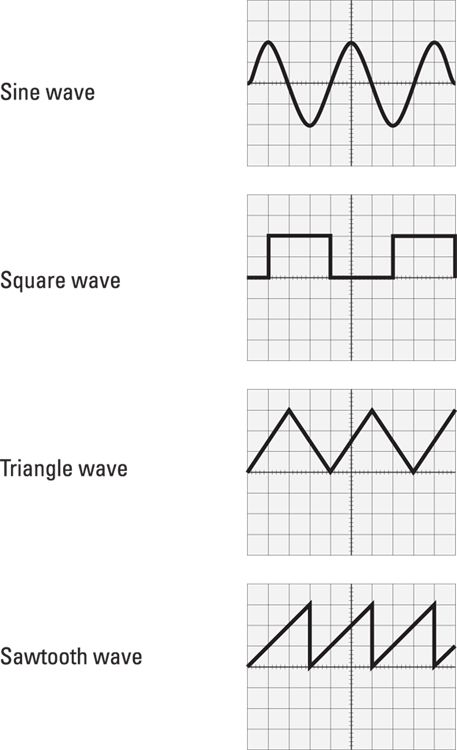
There are four basic types of waveforms that you’ll run into over and over again as you work with electronic circuits. These four waveforms are shown in Figure 9-3 . They are:

Sine wave: The voltage increases and decreases in a steady curve. If you remember your trigonometry class from high school, you might remember a trig function called sine , which has to do with angles measured in right triangles.

Few of us want to go back to high school trigonometry, so that’s all I’m going to say about the mathematics behind sine waves. Suffice it to say, however, that sine waves are found everywhere in nature. For example, sine waves can be found in sound waves, light waves, ocean waves — even the bouncing of a slinky is a sine wave.

And, most importantly from the standpoint of electronics, the alternating current voltage that is provided in the public power grid is in the form of a sine wave. In an alternating current sine wave, voltage increases steadily until a peak voltage is reached. Then, the voltage begins to decrease until it reaches zero. At that point, the voltage becomes negative, which causes the current flow to reverse direction. Once it’s negative, the voltage continues to change until it reaches its peak negative voltage, and then it begins to increase until it reaches zero again. The voltage then becomes positive, the current reverses, and the sine wave cycle repeats.

The number of times a sine wave (or any other wave, for that matter) repeats itself is called its frequency. Frequency is measured in units called hertz , abbreviated Hz. The alternating current available from a standard electrical outlet changes 60 times a second. Thus, the frequency of household AC is 60 Hz. Most waveforms found in electronic circuits have a much higher frequency than household alternating current, typically in the range of several thousand hertz (kilohertz, or kHz ) or millions of hertz (megahertz , or MHz ).
Square wave: Represents a signal in which a voltage simply turns on, stays on for awhile, turns off, stays off for awhile, and then repeats. The graph of such a wave shows sharp, right-angle turns, which is why it’s called a square wave.

In actual practice, most circuits that attempt to create square waves don’t do their job perfectly. As a result, the voltage rarely comes on absolutely instantly, and it rarely shuts off absolutely instantly. Thus, the vertical parts of the square wave in Figure 9-3 aren’t actually vertical in the real world. In addition, sometimes the initial voltage overshoots the target voltage by a little bit, so the initial vertical uptake goes a little too high for a very brief moment, and then settles down to the right voltage.

Square waves are found in many electronic circuits. For example, the 555 timer IC used in the coin-toss project presented in Chapter 6 of this minibook produces square waves that flash the light-emitting diodes on and off, and digital logic circuits (for example, computer circuits) rely almost exclusively on square waves to represent the ones and zeros of digital electronics. (I tell you more about the 555 timer IC in Book 3, Chapter 2 , and digital electronics in Book 5 .
Triangle wave: Voltage increases in a straight line until it reaches a peak value, and then it decreases in a straight line. If the voltage reaches zero and then begins to rise again, the triangle wave is a form of direct current. If the voltage crosses zero and goes negative before it begins to rise again, the triangle wave is a form of alternating current.
Sawtooth wave: This one is a hybrid of a triangle wave and a square wave. In most sawtooth waves, the voltage increases in a straight line until it reaches its peak voltage, and then the voltage drops instantly (or as close to instantly as possible) to zero, and immediately repeats.

Sawtooth waves have many interesting applications. One of the most appropriate for the purposes of this chapter is within an oscilloscope that has a CRT display. Here’s a very simplified explanation of how the CRT in an oscilloscope works: It shoots a beam of electrons at a specially coated glass surface that glows when electrons hit it and uses electromagnets to steer the beam. Electromagnets above and below the beam steer it vertically; electromagnets to the right and left steer it horizontally.

To create the sweep of the electron beam from left to right, a sawtooth wave is applied to the electromagnets on the left and right of the beam. As the voltage increases, the electromagnet produces an increasingly stronger magnetic field, which pulls the beam toward the right side of display. When the voltage reaches its peak and drops instantly back to zero, the magnetic field collapses, and the electron beam snaps back to the left side of the display.

Changing the sweep rate of the oscilloscope is simply a matter of changing the frequency of the sawtooth wave applied to the horizontal electromagnets in the oscilloscope’s CRT.

Calibrating an Oscilloscope

Quick: What were the first words spoken from the surface of the moon?

If you guessed, “That’s one small step for a man,” you’d be off by a long shot. Neil Armstrong and Buzz Aldrin had been on the moon for several hours by the time Neil said that.

If you guessed, “Houston, Tranquility Base here; the Eagle has landed,” you’d be close, but still not quite right.

Contrary to popular belief, the first words spoken from the surface of the moon were not spoken by Buzz Aldrin, not Neil Armstrong. Those first words were: “Engine Stop. ACA out of detent. Auto mode control, both auto. Descent engine command override, off. Engine arm, off. 413 is in.”

Before Neil Armstrong could make his historic announcement that the Eagle had landed on the moon, Buzz (being the lunar module pilot) had to quickly verify the settings of some key controls within the lunar module to ensure that everything was working well.

In the same way, before you make your historic first waveform measurement, you must first verify the settings of some key controls on your oscilloscope to ensure that everything is working well. The exact steps you need to follow to set up your oscilloscope vary depending on the exact type and model of your scope, so be sure to read the instruction manual that came with your scope. But the general steps should be as follows:

Examine all the controls on your scope and set them to normal positions.

For most scopes, all rotating dials should be centered, all push buttons should be out, and all slide switches and paddle switches should be up.
Turn your oscilloscope on.

If it’s the old-fashioned CRT kind, give it a minute or two to warm up.
Set the VOLTS/DIV control to 1.

This sets the scope to display one volt per vertical division. Depending on the signal you’re displaying, you may need to increase or decrease this setting, but one volt is a good starting point.
Set the TIME/DIV control to 1 ms.

This control determines the time interval represented by each horizontal division on the display. Try turning this dial to its slowest setting. (On my scope, the slowest setting is half a second, so it takes a full 5 seconds for the dot to travel across the screen.) Then, turn the dial one notch at a time and watch the dot speed up until it becomes a solid line.
Set the Trigger switch to Auto.

The Auto position enables the oscilloscope to stabilize the trace on a common trigger point in the waveform. If the trigger mode isn’t set to Auto, the waveform may drift across the screen, making it difficult to watch.
Connect a probe to the input connector.

If your scope has more than one input connector, connect the probe to the one labeled A.

Oscilloscope probes include a probe point, which you connect to the input signal and a separate ground lead. The ground lead usually has an alligator clip. When testing a circuit, this clip can be connected to any common ground point within the circuit. In some probes, the ground lead is detachable, so you can remove it when it isn’t needed.
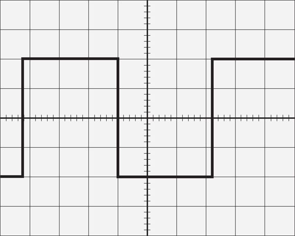
Touch the end of the probe to the scope’s calibration terminal.

This terminal provides a sample square wave that you can use to calibrate the scope’s display. Some scopes have two calibration terminals, labeled 0.2 V and 2 V. If your scope has two terminals, touch the probe to the 2 V terminal.

For calibrating, it’s best to use an alligator clip test probe. If your test probe has a pointy tip instead of an alligator clip, you can usually push the tip through the little hole in the end of the calibration terminal to hold the probe in place.

It isn’t necessary to connect the ground lead of your test probe for calibration.
If necessary, adjust the TIME/DIV and VOLTS/DIV controls until the square wave fits nicely within the display.

For example, see Figure 9-4 .
If necessary, adjust the Y-POS control to center the trace vertically.
If necessary, adjust the X-POS control to center the trace horizontally.
If necessary, adjust the Intensity and Focus settings to get a clear trace.
Congratulate yourself!

You’re now ready to begin viewing the waveforms of actual electronic signals.

FIGURE 9-4: An oscilloscope trace showing a square wave.

Remember that the controls of every oscilloscope make and model are unique. Be sure to read the owner’s manual that came with your oscilloscope to see if there are any other setup or calibration procedures you need to follow before feeding real signals into your scope.

Displaying Signals

The basic procedure for testing a circuit with an oscilloscope is to attach the ground connector of the scope’s test lead to a ground point in the circuit, and then touch the tip of the probe to the point in the circuit that you want to test.

For example, if you want to verify that the output from a pin of an integrated circuit is emitting a square wave, touch the oscilloscope probe to the pin and look at the display on the scope. Note that you may need to adjust the VOLTS/DIV and TIME/DIV settings on the scope to clearly see the waveform. But once you get those settings adjusted correctly, you should be able to visualize the square wave. If the square wave doesn’t appear, you likely have a problem with the circuit.

Never connect the oscilloscope probe directly to an electrical outlet. You’re likely to kill your scope or yourself. (If you want to measure voltage from an outlet, just use your regular multimeter.)

The following paragraphs give a few ideas for viewing various kinds of waveforms with an oscilloscope:

To view a simple DC waveform, try connecting the oscilloscope to a 1.5 V battery such as a AA or AAA cell. Set the VOLTS/DIV knob to 2 V, and then touch the probe ground connector to the negative battery terminal and the probe tip to the positive terminal. The resulting display should be a simple straight line midway between the second and third vertical division above the centerline. (If the battery is dead or weak, this line may be lower.)
If you want to see the 60 Hz sine wave available from an electrical wall outlet, find a plug-in power supply (commonly called a wall wart) that generates low-voltage AC. If you don’t have one lying around, you can buy them new at many stores. You can also find them for $1 or so at thrift stores. Plug the wall wart into an electrical outlet, and then connect the oscilloscope probe to the wall wart’s low-voltage plug. Adjust the VOLTS/DIV and TIME/DIV settings until you can see the sine wave.
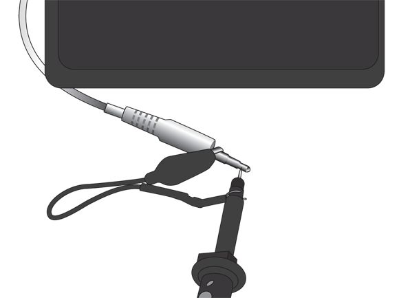
If you want to see what an audio waveform looks like, find a short -inch audio cable that’s male on both ends. Plug one end into the headphone jack of any audio device, such as a radio or an iPod. Then, connect the probe’s ground lead to the shaft of the plug on the free end of the audio cable and touch the probe tip to the tip of the audio plug, as shown in Figure 9-5 . After fiddling with the VOLTS/DIV and TIME/DIV settings, you should see a display of the jumbled waveform that’s typical of audio signals.
As you build circuits while working your way through this book, keep your oscilloscope handy. Don’t hesitate at any time to pick up the oscilloscope probe and check out the signals that are being generated at various points within your circuit. Connect the probe’s ground clip to any ground point in the circuit, and then touch the probe tip to every loose wire and exposed pin that you can to see what’s going on inside the circuit.

FIGURE 9-5: Connecting an oscilloscope probe to an audio plug.