5
Effect of Nano-Cages on Vibration
The infrared spectra of carbon dioxide (CO2) and nitrous oxide (N2O, dinitrogen monoxide) molecules, components of the Earth’s atmosphere, are well known in the gas phase. In a solid medium, similar to the crystalline lattice of a rare gas matrix, the nano-cage, a single or double substitution site that contains the molecule, is a region of a force field that is no longer isotropic, like in a vacuum. This results in a 5% relative shift of the vibrational frequencies and a change in the movements relative to the translational degrees of freedom of the center of mass and the overall rotation of the molecule. The frequency spectrum of the linear molecule then consists of a low-frequency IR component and a high-frequency vibrational IR component. This results in a modification of the thermal properties of the matrix– molecule system and when this system absorbs energy in the form of IR radiation by the molecule in the matrix, the de-excitation leads to different phenomena, either a radiative relaxation or a non-radiative relaxation or a mixture of both de-excitation pathways. These energy transfers are of particular importance in the interstellar medium or the interstellar space, since the absorption of IR radiation and the restitution of this energy can have an influence on the subsequent evolution of the physicochemical system in the immediate environment.
5.1. Introduction
The application of the theoretical inclusion model described in Chapter 4 by means of a program written in the FORTRAN language showed how to numerically determine the equilibrium configuration of the noble gas molecule–matrix system in the case of the C3 molecule in its linear and nonlinear form as well as in the case of the nonlinear molecule O3. The same procedure is used for the linear CO2 and N2O molecules. Modeling the effects of the medium on the various degrees of freedom of movement of the trapped molecule makes it possible to calculate the energy levels associated with these different degrees of freedom, whether it is the high-frequency vibrations of the nuclei, the perturbed rotation or the libration of the molecular structure as a whole or the bounded translation or vibration of its center of mass. The links between the degrees of freedom of the molecule and those of the host matrix can also be determined.
In Chapter 4, emphasis has been placed on low-frequency orientational modes that modify the thermal properties of the molecule–matrix system. In this chapter, the application of the model will be illustrated by the use of a program written in the MAPLE language, to calculate the vibrational frequency shifts in the case of CO2 and N2O molecules, this time focusing on the high-frequency vibrational modes. It is shown in particular that the perturbation of degenerate modes is a function of the symmetry of the trapping nano-site. Slow mode level diagrams will also be discussed with reference to the results given in Chapter 4.
5.2. The theoretical molecule–matrix model
The theoretical model was described in detail in Chapter 4, Volume 1 [DAH 17] and also revisited in Chapter 4 of this volume illustrated by programs written for numerical computation. The MAPLE program, which is described in the chapter, following the application of the theoretical model in the preceding chapter, makes it possible to analytically calculate the effect of the noble gas matrix on the vibrational modes. The complete program is given in the Appendix. It can be applied to noble gas matrices or to a nano-cage of a condensed-phase medium such as, for example, the case of clathrate cages discussed in Chapter 3 of this volume.
In this chapter, we explain the different parts of the MAPLE program so that its application by the reader is facilitated by referring to the different aspects of the model, which are:
- 1) the inclusion model which locally limits the movements of the molecule in a crystal lattice deformed by it;
- 2) the calculation of the potential interaction energy of the molecule–matrix system by a Lennard-Jones 12-6 potential, and a polarization energy of the atoms;
- 3) the calculation of the distortion of the atoms in the surrounding medium around the trapped molecules;
- 4) taking into account the decoupling of slow modes ((ωQ), perturbed rotation or libration of the molecular structure as a whole, bounded translation or vibration of the center of mass) by fixing the molecule in the position determined by the program given in Chapter 4, in order to focus on the fast modes (high-frequency vibrations (ωq) of the atoms of the molecule).
5.3. Calculation of the shift of vibrational frequencies
In the IR domain, the matrix vibrational frequency shifts were first qualitatively interpreted by Pimentel and Charles [PIM 63] in terms of rigid nano-cage for blue shift and soft nano-cage for red shift. At low temperatures, in a noble gas matrix, only the fundamental modes and some rare combination modes are present in the experimental IR spectra. The matrix effect on the vibrations can be determined by adjusting the force constants [Appendix 5.5.1] to fit the calculated frequency values to the observed ones. This technique was applied to study the triatomic ClCN and N2O molecules in Ar, Ne and CH4 [MUR 71a, MUR 71b] and N2 [SMI 72] matrices, respectively. The authors of references [MUR 71a, MUR 71b] and [SMI 72] come to the conclusion that only the constants of harmonic forces are significantly modified by the matrices.
Theoretical models that have been developed to study diatomic molecules have already been described in Chapter 4 of Volume 1 [DAH 17] and in Chapter 4 of this volume, for crystalline systems not deformed by the inclusion of the diatomic molecule. Buckingham [BUC 58, BUC 60a, BUC 60b] determined shifts by applying the perturbation theory up to second-order, and Charles and Lee [CHA 65], by applying this method, showed that the CO rotation is affected in the matrix. It is necessary to take into account the distortion of the matrix for the calculations to be valid. The distortion of the solid matrix environment is taken into account in the models developed by Kono and Lin [KON 83, KON 84] to study hydracids, and Girardet and Lakhlifi to study NH3 [GIR 85, GIR 86, GIR 89a, GIR 89b] and CH3F [LAK 89]. It is calculated by applying the Green’s crystal function technique as described in Volume 1 [DAH 17] and Chapter 4.
This inclusion model, which combines analytical and numerical methods, has been applied to the triatomic molecules O3 [LAK 93] and C3 [LAK 97]. It was then reformulated to calculate the vibrational shifts by introducing the matrix effect as a perturbation in the formalism applied to gas-phase molecules (equation [4.9] of Chapter 4). This extended model of Lakhlifi–Dahoo [DAH 97, DAH 99a, DAH 99b] makes it possible to determine the effect of a nano-cage (substitution site in a matrix or clathrate, fullerene or zeolite nano-cage) on the vibration of a molecule, by calculating the effect of the electromagnetic field present in the cage on the electronic potential driving the movement of the nuclei of the molecule, taking into account the symmetry of both the nano-cage and the molecule.
5.3.1. Calculation principle
Studying the IR spectroscopy of solid-phase CO2 and N2O linear molecules is possible by treating both the anharmonic contribution of the electronic potential, which drives the movement of the nuclei of the molecule during the vibration, and the matrix effect as a perturbation to the zero-order Hamiltonian of the gas phase (equation [4.9] of Chapter 4). Molecular methods based on contact transformation can then be applied to calculate the vibrational frequency displacement in the condensed phase.
Vibrational frequency shifts are calculated using the Born–Oppenheimer approximation. The decoupling of the internal degrees of freedom (the high-frequency modes which concern the vibrations of the molecule) and the external degrees of freedom (the low-frequency modes associated with the libration or the perturbed rotation, the translation movement of the center of mass and the vibrational motion of the atoms of the solid matrix) is a valid approximation in that the ratio of the frequencies associated with the internal modes to the highest frequency of the external modes is greater than 10 (except that for the lowest vibrational frequency, which is around 7) and because the symmetry of the internal modes does not coincide with those of the external modes and a dephasing phenomenon renders the coupling negligible.
It is necessary to choose the reference frame related to the equilibrium configuration of the molecule, to study vibrational movements, and thus to determine the interaction potential in this reference frame. To decouple vibrational movements from those linked to translation and rotation (or perturbed rotation or libration), the origin of the reference frame linked to the molecule (mobile reference frame) must coincide with its center of mass (Eckart conditions).
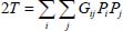
On the contrary, since the vibrational motions are associated with the normal coordinates, the potential must be expressed as a function of these normal coordinates, so that the vibrational frequencies of the molecule are expressed in the following form, in the harmonic approximation (Appendix 5.5.1):

where Qk are the normal coordinates of vibrational mode k and  is related to the frequency ωk of this mode of vibration.
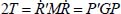
At the harmonic approximation, the kinetic energy operator is diagonal as a function of normal coordinates (Appendix 5.5.1):
where Mi is the mass of the atom i, (xi, yi, zi) are the Cartesian coordinates of this atom and Qk are the normal vibrational coordinates.
The short- and medium-range interactions between an atom i of the molecule and an atom j of the solid matrix are modeled by the sum of a Lennard-Jones potential and a potential taking into account the polarization of the matrix atoms by the trapped molecule. The matrix effect is calculated for the vibrational levels from the atom–atom potential expressed in the crystal-bound fixed reference frame as:
Since the distortion of the crystal is calculated in the absolute reference with center O (X, Y, Z), it is necessary to define the interaction potential in the reference frame of the molecule to calculate the vibration of the atoms of this molecule. It is also necessary to calculate the electric field corresponding to the induced dipole-dipole interaction.
In the mobile coordinate system, the vibration of atom i is defined by the position vector  . The distance vector
  between atom i of the molecule and atom j of the crystal is decomposed in the following form:
where M is the rotational unit transformation matrix [ROS 67] which makes it possible to move from the position vector  expressed in the coordinate system bound to the crystal to the position vector
  expressed in the reference frame linked to the molecule.
When the trapped molecule vibrates, the atom i moves with respect to its equilibrium position (defined by  ). The distance vector in this case is composed of a term related to the equilibrium configuration of the atom i and a term
  related to the movement of the latter with respect to its equilibrium position, that is:

We can write:
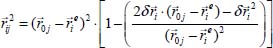
Assuming that the displacement vector is small with regard to  , we can develop the expression of the equation [5.3] as a second-order Taylor series, that is, using the following expansion:
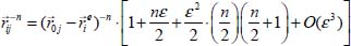
where:
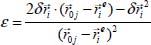
with n = 12 and n = 6 to determine the interaction potential as a function of the displacement vector . The potential is then expressed as a function of normal dimensionless coordinates {qν}, from a change of basis from Cartesian coordinates to normal coordinates (Appendix 5.5.1).
The induction potential is also expanded according to dimensionless normal coordinates {qν}. We find that among the set of multipolar moments that make up the electrostatic field, only the dipole moments polarize the atoms of the noble gas matrix.
From the equilibrium configurations, determined for CO2 (single site and double site) and N2O (double site), and taking into account the expansion of the interaction potential between the molecule and the matrix, as a function of dimensionless normal coordinates, we obtain:

In equation [5.9], only a perturbation up to the second-order is taken into account. Once this potential is obtained, it is considered as a perturbation of the Hamiltonian of the isolated molecule (equation [4.9] of Chapter 4).
5.3.2. Application of the MAPLE program
5.3.2.1. The site inclusion model
The noble gases which crystallize according to a face-centered cubic system (fcc) trap the triatomic molecules in two types of sites: single or double substitution sites. The equilibrium configuration is determined using the program described in Chapter 4.
Given their respective sizes (Table 4.3 in Chapter 4), the molecules O3, N2O and CO2 are substituted with one or two atoms in a site of symmetry Oh and D2h, respectively, in the fcc lattice and in some cases, that of a hexagonal close-packed (hcp) structure [LAK 93, DAH 97, DAH 99a, DAH 99b, LAK 00]. The position of the molecule is fixed in the nano-site before calculating the effect of the condensed phase on the vibrational modes.
5.3.2.2. Position of the molecule at equilibrium configuration in an argon matrix
To determine the vibrational movements of the molecule, under the influence of the matrix, it is appropriate to work in the frame of reference related to the equilibrium configuration of the molecule. The initial position of the molecule is that corresponding to the Oz axis of the mobile coordinate system coinciding with the internuclear axis. Then, we use the rotation matrix (Rose Convention) to bring the molecule to the calculated position by rotating the atoms of the crystal. The values of Euler angles previously calculated with the program described in Chapter 4 are used to determine the equilibrium configurations of the matrix–molecule system.
The following code written in the MAPLE language allows this initialization:
#####################################################################
# EULER ANGLES f for Phi, t for Theta and k for Khi (k = 0 if XYZ molecule is linear)
# VALUES FIXED TO THE EQUILIBRIUM CONFIGURATION
#####################################################################
f:=0.;
t:=evalf(Pi/2.);
k:=0.;
#####################################################################
# EQUILIBRIUM COORDINATES OF CO2
# POSITION OF ATOMS (O, C and O)
# VERTICAL AXIS Oz = INTERNUCLEAR AXIS
#####################################################################
X1:=0.;
Y1:=0.;
Z1:=-1.16;
X2:=0.;
Y2:=0.;
Z2:=0.;
X3:=0.;
Y3:=0.;
Z3:=1.16;
#####################################################################
… …
# ATOMS IN THE MOBILE REFERENCE FRAME BOUND TO THE MOLECULE
#####################################################################
G1:=vector([X1,Y1,Z1]);
G2:=vector([X2,Y2,Z2]);
G3:=vector([X3,Y3,Z3]);
GM1:=eval(G1);
GM2:=eval(G2);
GM3:=eval(G3);
#####################################################################
# ROTATIONAL MATRIX FROM ONE AXIS SYSTEM TO ANOTHER
# ROSE CONVENTION
#####################################################################
Cfi:=evalf(cos(f));
Sfi:=evalf(sin(f));
Cte:=evalf(cos(t));
Ste:=evalf(sin(t));
Cki:=evalf(cos(k));
Ski:=evalf(sin(k));
ROS:=matrix(3,3,[Cfi*Cte*Cki-Sfi*Ski,Sfi*Cte*Cki+Cfi*Ski,-Ste*Cki,
-Cfi*Cte*Ski-Sfi*Cki,-Sfi*Cte*Ski+Cfi*Cki,Ste*Ski,Cfi*Ste,Sfi*Ste,Cte]);
ROSE:=evalm(ROS);
#####################################################################
# POSITION VECTOR OF THE MATRIX ATOM IN THE MOBILE SYSTEM
# PROJECTION IN THE MOBILE FRAME IN THE ATOM POSITION
# FOR COMPONENTS OF THE POSITION VECTOR
######################################################################
RMj:=multiply(ROSE,RCj);
rojx:=dotprod(RMj,ex);
rojy:=dotprod(RMj,ey);
rojz:=dotprod(RMj,ez);
rojn:=norm(RMj,2);
#####################################################################
… …
5.3.2.3. Calculation of atom–atom parameters in an argon matrix
Calculating the Lennard-Jones (12-6) atom–atom potential requires determining the atom–atom parameters (Berthelot–Lorentz rules) from the intrinsic parameters (Table 4.2 in Chapter 4) of each atom before applying the formulae from equations in Chapter 4 (equations [4.2] and [4.4]).
The atom–atom parameters in an argon matrix are calculated according to the following code:
#####################################################################
# LENNARD-JONES PARAMETERS OF Ar-CO2 (EPSILON,SIGMA) C, O and O
# Polarizability of the Ar matrix
#####################################################################
alpha:=1.64;
e2j:=50.03;
e1j:=57.90;
e3j:=e1j;
sig2j:=3.329;
sig1j:=3.165;
sig3j:=sig1j;
else
… …
#####################################################################
5.3.2.4. Matrix effect on the potential as a function of normal coordinates
The matrix effect is calculated on the vibrational levels from the atom–atom potential expressed in the crystal-bound fixed reference frame. The transition from Cartesian coordinates to normal coordinates expresses this effect according to normal coordinates.
#####################################################################
# READING THE CHANGE OF BASIS
# CARTESIAN COORDINATES IN THE MOBILE REFERENCE FRAME
# FOR THE TRANSFORMATION INTO NORMAL COORDINATES
# SUDIVISION OF THE MATRIX INTO 3 3X4 MATRICES
######################################################################
readlib(readdata):
TRQ:=matrix(9,4,(readdata(LikW,4))):
TRQ1:=submatrix(TRQ,1..3,1..4);
TRQ2:=submatrix(TRQ,4..6,1..4);
TRQ3:=submatrix(TRQ,7..9,1..4);
Q1:=q1*BETA1;
Q21:=q2*BETA2;
Q22:=q3*BETA2;
Q3:=q4*BETA3;
Q:=matrix(4,1,[Q1,Q21,Q22,Q3]);
#####################################################################
# READING THE CHANGE OF BASIS
# CARTESIAN COORDINATES IN THE MOBILE REFERENCE FRAME
# FOR THE TRANSFORMATION INTO NORMAL COORDINATES
# SUDIVISION OF THE MATRIX INTO 3 3X4 MATRICES
######################################################################
M1:=evalm(TRQ1&*Q);
M2:=evalm(TRQ2&*Q);
M3:=evalm(TRQ3&*Q);
MV1:=subvector(M1,1..3,1);
MV2:=subvector(M2,1..3,1);
MV3:=subvector(M3,1..3,1);
PSMR1:=dotprod(MV1,Rj1);
PSMR2:=dotprod(MV2,Rj2);
PSMR3:=dotprod(MV3,Rj3);
M1ca:=dotprod(MV1,MV1);
M2ca:=dotprod(MV2,MV2);
M3ca:=dotprod(MV3,MV3);
#####################################################################
5.3.2.5. Calculation of the energy of the argon molecule–matrix system
The application of the formulae given in equations [4.2] and [4.4] of Chapter 4 allows us to calculate the energy of the molecule–matrix system. Equations [5.6] to [5.8] show how the vibrations of the molecule in the nano-site are taken into account. The transition from Cartesian coordinates to normal coordinates then makes it possible to determine the effect of the matrix on the internal vibrations of the molecule.
This calculation, for example, is carried out according to the following code:
#####################################################################
# ELECTRIC FIELD VECTOR COMPONENTS OF THE ELECTRIC DIPOLE
# AS A FUNCTION OF NORMAL COORDINATES
# INDUCED DIPOLE-DIPOLE INTERACTION ENERGY
######################################################################
Ejxmux:=(3*(rojx*rojx)-rojn^2)*mux/rojn^5;
Ejymux:=3*(rojy*rojx)*mux/rojn^5;
Ejzmux:=3*(rojz*rojx)*mux/rojn^5;
Ejxmuy:=3*(rojx*rojy)*muy/rojn^5;
Ejymuy:=(3*(rojy*rojy)-rojn^2)*muy/rojn^5;
Ejzmuy:=3*(rojz*rojy)*muy/rojn^5;
Ejxmuz:=3*(rojx*rojz)*muz/rojn^5;
Ejymuz:=3*(rojy*rojz)*muz/rojn^5;
Ejzmuz:=(3*(rojz*rojz)-rojn^2)*muz/rojn^5;
Exj:=Ejxmuz+Ejxmuy+Ejxmux;
Eyj:=Ejymuz+Ejymuy+Ejymux;
Ezj:=Ejzmuz+Ejzmuy+Ejzmux;
E2:=(Exj*Exj)+(Eyj*Eyj)+(Ezj*Ezj);
Vind:=-(1/2.)*5030.*alpha*E2;
Vindj:=expand(Vind);
#####################################################################
# POSITION VECTOR OF MATRIX ATOMS
# IN THE MOBILE REFERENCE FRAME BOUND TO THE MOLECULE
# CALCULATION OF NORMS
# ######################################################################
Rj1:=evalm(RMj-GM1);
Rj2:=evalm(RMj-GM2);
Rj3:=evalm(RMj-GM3);
NR21:=norm(Rj1,2);
NR22:=norm(Rj2,2);
NR23:=norm(Rj3,2);
NRj21:=eval(NR21);
NRj22:=eval(NR22);
NRj23:=eval(NR23);
#####################################################################
… ….
#####################################################################
# SECOND ORDER DEVELOPMENT OF THE ATOM-ATOM POTENTIAL
# AS A FUNCTION OF THE DISPLACEMENTS OF THE MOLECULE ATOMS
# DURING VIBRATION
# CARTESIAN COORDINATES IN THE MOBILE REFERENCE FRAME
######################################################################
esig1:=e1j*sig1j^n;
esig2:=e2j*sig2j^n;
esig3:=e3j*sig3j^n;
eps1:=(2*(PSMR1)-M1ca)/NRj21^2;
eps2:=(2*(PSMR2)-M2ca)/NRj22^2;
eps3:=(2*(PSMR3)-M3ca)/NRj23^2;
epss1:=(2*(PSMR1))/NRj21^2;
epss2:=(2*(PSMR2))/NRj22^2;
epss3:=(2*(PSMR3))/NRj23^2;
Vr1jn:=4*esig1*NRj21^(-n)*(1+1/2*n*eps1+1/2*(epss1^2)*((-n/2)*(-n/2-1))):
Vr2jn:=4*esig2*NRj22^(-n)*(1+1/2*n*eps2+1/2*(epss2^2)*((-n/2)*(-n/2-1))):
Vr3jn:=4*esig3*NRj23^(-n)*(1+1/2*n*eps3+1/2*(epss3^2)*((-n/2)*(-n/2-1))):
n:=6;
Vrij6:=eval(Vr1jn+Vr2jn+Vr3jn):
n:=n+6;
Vrij12:=eval(Vr1jn+Vr2jn+Vr3jn):
V:=-1.*Vrij6+Vrij12+Vindj:
Vj:=expand(V):
end:
#####################################################################
5.4. Application to linear triatomic molecules
The theoretical model described in the previous sections and in Chapter 4 of Volume 1 [DAH 17] was applied to the linear triatomic molecules CO2 and N2O [DAH 99a, DAH 99b, LAK 00, DAH 06]. The programs used to calculate the site distortion and the equilibrium configuration of the molecule in the nano-cage are given in the Appendix of Chapter 4.
5.4.1. Experimental study of linear triatomic molecules (CO2, N2O)
The inserted molecules are identified by their absorption spectra which are in the form of a Q* branch without rotational structure in the case of CO2 and N2O. In the case of CO2, for a resolution between 0.5 cm–1 and 1 cm–1, two absorption lines are observed per vibrational mode in argon. The antisymmetric vibrational mode and the degenerate mode ν2 appear as a doublet in the IR spectra. The mode ν3 has a peak at 2,339.0 cm–1 (low-frequency (LF) component) and 2,345.1 cm–1 (high-frequency (HF) components) with a standard deviation of 6.1 cm–1, and the mode ν2 peaks at 663.4 cm–1 (LF component) and at 665.0 cm–1 (HF component) with a standard deviation of 1.6 cm–1 [FRE 74, GUA 78, IRV 82, NXU 94]. At a better resolution, 0.15 cm–1, the HF component of the mode appears in the form of a doublet separated by 0.4 cm–1 for the isotopes 626 (16O 12C16O), 627 (16O12C 17O), 628 (16O12C 18O), 727 (17O 12C17O), 728 (17O12C 18O) and 636 (16O 13C16O) (see Figure 2 in [DAH 99]).
The work of Guasti et al. [GUA 78] on the monomers and dimers of the 12CO2 carbon dioxide molecule in noble gas matrices made it possible to identify the existence of two sites of different stabilities, after a strong annealing of the matrix (temperature increase beyond T = 35 K, then cooling). For each mode, one of the lines disappears after this strong annealing; the disappearing trapping site is termed an unstable site. Further work on monomers of the isotopes 636, 628 and 638 by Irvine et al. [IRV 82] allowed them to propose a structure for trapping sites based on qualitative considerations according to the distance between the oxygen atoms of the molecule and the argon atoms. The unstable site was identified as a single substitution site (S1: the molecule replaces an argon atom) and the stable site as a double substitution site (S2: the molecule replaces two argon atoms). The work presented in the reference [DAH 99a, DAH 99b] corrected this attribution thanks to the comparison between the calculations of the bar spectra from the extended Lakhlifi–Dahoo model and the experimental results. The calculations showed that a degeneracy lifting of the mode ν2 occurred in the S2 site. The annealing experiment showed that the LF line of mode ν3 is correlated with the HF line of mode ν2. This made it possible to confirm that the stable site was the single site S1 and that the unstable site was the double site S2. Annealing at a temperature below T = 25 also showed that both sites remained after annealing, meaning that, in this case, both are stable.
In the argon matrix, we note the presence of two trapping sites, a single nano-site (unstable if the annealing is strong) and a double nano-site (stable and persists after annealing). However, only one substitution site is observed in krypton and xenon matrices (single site S1). Similarly, a single line for N2O is observed in the argon matrix as a result of a single double trapping site (identified by the degeneracy lifting of the mode ν2).
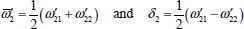
5.4.2. Frequency shift calculation for degenerate mode ν2
The originality of the developed theoretical model, for calculating vibrational shifts [DAH 99a, DAH 99b], is the possibility of applying the formalism developed in molecular physics to study the gas phase of molecules to these molecules when they evolve under the influence of the electromagnetic field present in a given environment, like the nano-site of a noble gas matrix (equations [4.9], [4.10a], [4.10b], [4.13a] and [4.13b] in Chapter 4). Studying the IR spectroscopy of solid-phase linear molecules CO2 and N2O is possible by calculating both the anharmonic contribution of the electronic potential which drives the movement of the nuclei of the molecule during the vibration and the matrix effect as a perturbation to the zeroth-order Hamiltonian of the gas phase (equation [4.9] in Chapter 4).
For molecules such as CO2 and N2O trapped in a double site, the zeroth-order Hamiltonian contains four non-degenerate vibrational modes due to the matrix effect and it is not possible to directly apply the methods used in the gas phase. Indeed, a linear molecule that has four normal non-degenerate vibrational modes does not exist in the gas phase. In the reference [DAH 99], it is shown how to calculate the effect of the single site S1 and the double site S2 in the same manner by transforming the zeroth-order Hamiltonian of the molecule trapped in the double S2 site as follows:
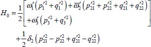
with
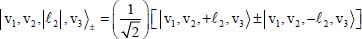
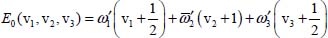
The first term on the right-hand side of equation [5.10] corresponds to the zeroth-order Hamiltonian operator of a linear triatomic molecule with a degenerate vibrational mode of frequency  . The Hamiltonian operator is diagonal in Wang’s eigenvector basis [WAN 29] whose expressions are:
and the eigenenergy is given by:
The second term on the right-hand side of equation [5.10] is considered as a perturbation term V0 to the zeroth-order Hamiltonian. The non-diagonal matrix elements of V0 in Wang’s basis are given by:


For example, the degeneracy of the level |0,1, 1,0〉± is lifted by the perturbation V0. From equations [5.11], [5.14a] and [5.14b], the calculation of the two corresponding energies leads to:


These calculations were applied to the linear triatomic molecules CO2 and N2O, and the results are given in the references [DAH 99a, DAH 99b, LAK 00] for the argon matrix and [DAH 06] for the krypton and xenon matrices.
5.4.3. Calculation results for linear triatomic molecules (CO2, N2O)
5.4.3.1. Equilibrium configuration and molecule position in the matrix
The calculation methods described in Chapter 4 were applied to the linear triatomic molecules CO2 and N2O in matrices, by sampling the angular positions and the change in the center of mass position of the trapped molecule, in order to determine the potential energy hypersurface in which it evolves. Up to 32 layers of rare gas atoms can be considered, that is, 1,060 atoms. Studies show that the 10th layer (200 atoms) for the fcc crystal lattice is enough to reach a good convergence of results when calculating the energy of the molecule–matrix system. For the hcp structure, it is necessary to consider at least the 18th layer (206 atoms). In the fcc lattice, the molecule replaces the central atom in the single site or two adjacent atoms in the double site. These two nano-sites are characterized by different symmetries, Oh for S1 and D2h for S2.
In the single site S1, the Ar–CO2 matrix system potential curves as a function of θ (φ and  fixed), φ (θ and fixed) and (θ and φ fixed) show that minimal energy is obtained when θ = 0, that is, when the molecule is vertical and aligned with one of the C4 axes of symmetry of the matrix. The other stable configurations obtained for θ = π/2 and φ = 0 or π/2 always correspond to the case where the molecule axis is parallel to the C4 axes of the crystal, with the molecule’s center of mass coinciding with the center of the site, as shown in Figure 5.1. In the case of the molecule N2O, a single site does allow a negative energy configuration.
In a double site, minima are calculated for the angle θ = π/2, which corresponds to a position of the CO2 molecule in the alignment of two substituted argon atoms, that is, parallel to the C2 axis of symmetry of the site (angle φ = –π/4). In the case of the N2O molecule in a double site, the potential interaction energy is minimal when the molecule is in a similar position, that is, aligned with the C2 axis of symmetry (φ = –π/4) (Figure 5.1). The center of mass can move almost freely, about 1 Å and 2 Å for N2O and CO2, respectively, from the center of the site.
In krypton (Kr) and xenon (Xe) matrices, both sites have comparable energy minima values. The probability of trapping the molecule in both sites is slightly different. Let us note that experimentally, the molecule is trapped preferentially in a single substitution site S1 (absence of degeneracy of the mode ν2).

Figure 5.1. Possible trapping sites of CO2 and the equilibrium configuration in a fcc network. For a color version of this figure, see www.iste.co.uk/dahoo/infrared2.zip
Although the compact hexagonal lattice (i.e. the hcp) is less likely than the fcc one, since the energy difference between the two structures is about 600 cm–1, the calculations show that if the CO2 molecule replaces an atom in the center of the hexagon, an energy minimum is obtained for a molecule orientation parallel to the C3 axis of the site. The configuration corresponds to the parameters: θ= 0, φ = 0 and = 0 in the xenon and krypton matrices for which the energies are negative (in the argon matrix, the calculated energy is positive). As for the xenon matrix, the calculation shows that the trapping in each type of lattice (fcc and hcp) is possible because the energy difference is only about 200 cm–1. Consistent with the experiment, both hcp and fcc structures coexist when the deposition temperature is greater than or equal to 35 K [CHA 00].
5.4.3.2. Distortion of the rare gas matrix
The calculation of the distortion using Green’s functions leads to a local dilation of the argon matrix by 0.28 Å, that is, 7% of the diameter of the single site S1 for a displacement of the first eight atoms in the first layer of the cage. These atoms are contained in two perpendicular planes containing the molecule’s axis. The displacement of the other four atoms of the layer, which form another plane, does not exceed 10% of the previous value. These displacements correspond globally to the dilation of the cage around the CO2 molecule as shown in Figure 5.1. With the distortion of the two groups of atoms linked to the two perpendicular planes being equivalent, the effect on the vibrational mode ν2 on the degeneracy lift in the site S1 is negligible.
In the double site, the calculations show that two equilibrium positions are possible giving an energy minimum for the CO2 and N2O molecules. They are off-center with respect to the center of the site and can move freely along the symmetry axis C2 of the site. For vibrational shift calculations, the molecule will be clamped in one of the equilibrium positions. In the case of the molecule CO2, the maximum distortion is 0.11 Å (i.e. 1% of the diameter of the site). This distortion involves the four atoms around the center of the site, with the other atoms in the first layer being displaced by about 0.03 Å. A slight contraction of the atoms placed on the C2 axis of symmetry of the crystal is determined by the calculations. The anisotropic distortion of the double site makes its environment slightly asymmetrical, leading to the degeneracy lifting of mode ν2. In the case of the molecule N2O, the distortion corresponds to a dilation of the cage whose maximum displacement is 0.32 Å (i.e. 7% of the site diameter).
To adjust the vibrational shifts observed in the matrix with respect to the position of gas-phase transitions, it is necessary to numerically simulate a gradual distortion of the first four layers around the molecule (see program in Appendix 5.5.2). In the single site S1, the distortion of the cage leads to a 17% dilation of the first layer, 8% for the second, 4% for the third and finally, 2% for the fourth. In the double site, the dilation of the first four layers around the molecule is much smaller given the initial size of the site, 6%, 3%, 1.5% and 0.7%, respectively.
5.4.3.3. Matrix effect on potential as a function of normal coordinates
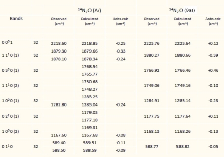
Determining the vibrational movements of the fundamental bands due to the matrix effect requires knowledge of the terms βν and βνν' and the molecule–matrix interaction potential (equation [5.9]). For calculations, the values of the vibrational potential constants of the gas phase are taken from the references [SUZ 68, TEF 90]. The results of the calculations are given in Tables 5.1 and 5.2 for the molecules CO2 (636) and N2O (646) in the argon matrix. They show that for the CO2 molecule, the observed vibrational displacements are essentially due to the changes in the harmonic constants, that there are two possible trapping sites and that the degeneracy of the vibrational mode ν2 is lifted in the double site S2. In the case of CO2, this amounts to assigning the double substitution site to the unstable site and the single site to the stable site, contrary to what Irvine et al. [IRV 82] stated. For N2O, there is only one trapping site. Since it is a double site (S2), a degeneracy lifting of mode ν2 is also expected.
The results of both Tables 5.1 and 5.2 show consistency between the observed and calculated values for linear CO2 and N2O molecules.
Table 5.1. Gas and matrix vibrational energies for 13C16O2 (cm–1)
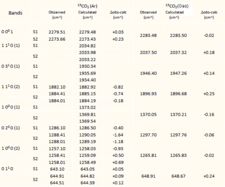
Table 5.2. Gas and matrix vibrational energies for 14N216O (cm–1)
5.4.3.4. Couplings between the molecule and the matrix
In the case of couplings between a linear or nonlinear triatomic molecule and a matrix, it is expected that they are different for the three molecules O3, CO2 and N2O as a result of the different physical characteristics (Table 5.3):
- – structures (linear for CO2 and N2O and nonlinear for O3);
- – dimensions and compositions (mass);
- – symmetry properties; and
- – electrical characteristics (quadrupole moment for CO2 and dipole moment for O3 and N2O).
The effects of different couplings with the different noble gas matrices (Ar, Kr and Xe) lead to a multiplicity of energy relaxation pathways in these matrices and consequently to different thermal properties.
Table 5.3. Parameters of the rigid molecule: r0 bond length (Å), β bond angle (degree), μ dipole moment (Debye) and Qii quadrupole moment according to the axis i of the molecule (Debye Å)
| ro(Å) | β (degrees) | μ(D) | Qzz (D Å) | Qxx (D Å) | Qyy (D Å) | |
| 16O3 | 1.278 | 116.8 | 0.532 | –1.4 | –0.7 | 2.1 |
| 13C16O2 | 1.16 | 180 | 0 | –4.3 | 2.15 | 2.15 |
| 14N216O | N-N: 1.128 N-O: 1.842 | 180 | 1.66 | –3.0 | 1.5 | 1.5 |
For example, analyzing the calculated potential curves shows that the coupling between the matrix and the CO2 molecule is weaker in the double site, which is compatible with the smaller linewidth of the mode ν3 for this site, γ = 0.13 cm–1, compared with γ = 0.40 cm–1 for the single site. On the contrary, if we compare the calculated potential curves for N2O and CO2, in the case of the double site, we note that some configurations of N2O lead to positive energy values, an order of magnitude higher than the well depth corresponding to the equilibrium position, whereas in the case of CO2, the calculated energies are always negative. It is expected that the matrix effect will be greater on N2O than on CO2 in the relaxation of the vibrational energy of these molecules. It is possible to calculate the shifts of the fundamental modes of vibration starting from the modification of the harmonic constants of the molecules CO2 and N2O, disregarding the possible modifications to the anharmonic constants by the matrix effect.
5.5. Appendices
5.5.1. Transition from Cartesian coordinates to normal coordinates
It is possible to express the harmonic potential according to the internal coordinates of the atoms in the molecule, in order to be able to use the properties of symmetry of the molecule within the context of group theory (Chapter 1 of this volume) and to then express this potential according to the normal coordinates. The transition from Cartesian coordinates to internal coordinates is relatively easy from the geometric equilibrium configuration of the molecule.
In terms of the internal coordinates Ri, the harmonic potential has the expression:
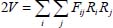
where Fij is the matrix of the force constants connected to the second derivatives of the potential.
For small atomic displacements, the kinetic energy can be written in the following form, according to the internal coordinates:
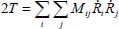
where Mij are the matrix elements connected to the atomic masses and whose structure is linked to the equilibrium geometry of the molecule and  corresponds to the derivative of the internal coordinate with respect to time.
It is more convenient for the transition from classical mechanics to quantum mechanics to express kinetic energy as a function of conjugate variables:
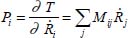
such that:
with:

These relations are written in the following form:


On the basis of the normal coordinates, the matrices of the kinetic energy operator T and potential energy operator V are diagonal. Internal coordinates are defined as linear combinations of normal coordinates as follows:
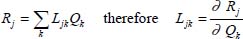
This transformation gives:


The parameter λk, proportional to the square of the frequency of the kth vibrational mode corresponds to each coordinate Qk, such as .
In terms of matrices, it becomes:


where Λ is a diagonal matrix whose elements are the parameters λk
By substituting [A5.9a] in [A5.6c] and [A5.6d] and comparing with [A5.9b] and [A5.9c], we find that:


By combining these two equations, we obtain the following forms:


These lead to the following relationships for the determinants:


The calculation of the normal coordinates is reduced to the calculation of a determinant once the elements Mij or Gij are determined.
We then use the symmetry coordinates, which are linear combinations of the internal coordinates based on the symmetry properties of the molecule, to simplify the calculation of the secular determinant.
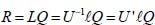
The transition from internal coordinates to symmetry coordinates takes place via matrix U and that from normal coordinates to symmetry coordinates by matrix ℓ:


Thus, we can determine the internal coordinates according to the normal coordinates as follows:
5.5.2. MAPLE program for displacement/shifts of vibrational frequency modes of a CO2 molecule in a noble gas nano-cage matrix
#####################################################################
# CALCULATING THE CHANGE IN ELECTRONIC POTENTIAL
# THAT CONTROLS VIBRATION OF A MOLECULE OF TYPE XYZ (O3, CO2, N2O…)
# TRAPPED IN A NOBLE GAS MATRIX IN A SINGLE SITE
#####################################################################
with(linalg):
#Digits:=30;
#####################################################################
# RESULTS COMPUTED USING A FORTRAN PROGRAM
#####################################################################
writeto(Bij1);
print(MATRICELikWilson);
#####################################################################
# SUB PROGRAM OF THE POTENTIAL CALCULATION
# THE INDEX « MATRIX » IS USED TO IDENTIFY THE MATRIX ATOMS
# IN CLATHRATES THE ATOMS ARE RANKED IN ORDER : O, H and H.
# 3 TRANSFORMATIONS ARE NEEDED FOR THE CLATHRATE SYSTEM (SITE S1 or S2)
# IN THE NOBLE GAS MATRIX THE ORDER CORRESPONDS TO A Ar, Kr and Xe
# 1 TRANSFORMATION IS REQUIRED FOR EACH MATRIX AND FOR EACH SITE SITE
#THE PROGRAM IS WRITTEN FOR THE MATRICES AND THE CO2 MOLECULE
#####################################################################
vpotj:=proc(RRj,matrix)
local e1j,e2j,e3j,sig1j,sig2j,sig3j,f,t,k,XCj,YCj,ZCj,X1,Y1,Z1,X2,Y2,Z2,X3,Y3,
   Z3,Cfi,Sfi,Cte,Ste,Cki,Ski,G1,G2,G3,GM1,GM2,GM3,RCj,ROS,ROSE,RMj,Rj1,Rj2,
   Rj3,NR21,NR22,NR23,NRj21,NRj22,NRj23,TRQ,TRQ1,TRQ2,TRQ3,Q,M1,M2,M3,MV1,MV2,
   MV3,PSMR1,PSMR2,PSMR3,M1ca,M2ca,M3ca,esig1,esig2,esig3,eps1,eps2,eps3,
   epss1,epss2,epss3,Vr1jn,Vr2jn,Vr3jn,n,Vrij6,Vrij12,V,Vj,VVj,
   alpha,cto,h,c,BETA,w10,w20,w30,BETA1,BETA2,BETA3,Q0,BE,RO1,
   CB,SB,A0,ex,ey,ez,mux,muz,muy,TG,ROT,RCTj,rojx,rojy,rojz,rojn,
   Ejxmux,Ejymux,Ejzmux,Ejxmuz,Ejymuz,Ejzmuz,Exj,Eyj,Ezj,E2,
   Vind,Vindj,Q1,Q21,Q22,Q3,Ejxmuy,Ejymuy,Ejzmuy;
with(linalg):
#Digits:=20;
RCj:=eval(RRj);
if matrix=1 then
#####################################################################
# LENNARD-JONES PARAMETERS Ar-CO2
#####################################################################
 alpha:=1.64;
 e2j:=50.03;
 e1j:=57.89;
 e3j:=e1j;
 sig2j:=3.329;
 sig1j:=3.165;
 sig3j:=sig1j;
 else
  if matrix=2 then
#####################################################################
# LENNARD-JONES PARAMETERS Kr-CO2
#####################################################################
  alpha:=2.48;
  e2j:=61.03;
  e1j:=70.62;
  e3j:=e1j;
  sig2j:=3.430;
  sig1j:=3.266;
  sig3j:=sig1j;
  else
#####################################################################
#	LENNARD-JONES PARAMETERS Xe-CO2
#####################################################################
  alpha:=4.04;
  e2j:=68.42;
  e1j:=79.17;
  e3j:=e1j;
  sig2j:=3.590;
  sig1j:=3.426;
  sig3j:=sig1j;
 fi;
fi;
#####################################################################
# EULER ANGLES f for Phi, t for Theta and k for Khi (k = 0 IF XYZ is linear)
# FIXED VALUES IN THE EQUILIBRIUM CONFIGURATION
# ALLOWS THE TRANSITION FROM THE MOBILE FRAME TO THE FIXED FRAME AND VICEVERSA
#####################################################################
f:=0.;
t:=evalf(Pi/2.);
k:=0.;
#####################################################################
# EQUILIBRIUM COORDINATES OF CO2
# POSITION OF ATOMS (O,C and O)
VERTICAL # AXIS Oz = INTERNUCLEAR AXIS
#####################################################################
X1:=0.;
Y1:=0.;
Z1:=-1.16;
X2:=0.;
Y2:=0.;
Z2:=0.;
X3:=0.;
Y3:=0.;
Z3:=1.16;
#####################################################################
# DEFINITION OF BASIS VECTORS OF THE MOBILE REFERENCE FRAME
#####################################################################
ex:=eval(vector([1,0,0]));
ey:=eval(vector([0,1,0]));
ez:=eval(vector([0,0,1]));
#####################################################################
# DIPOLE MOMENTS IF NON-ZERO (O3, C3, CO2,N2O)
# AS A FUNCTION OF NORMAL COORDINATES
# q1 symmetric vibration, zero
# q4 asymmetric vibratione, nu3
# q2 and q3 degenerate bending vibration nu2
#####################################################################
#muz:=0.448*q4-0.0177*q1*q4;
#####################################################################
# in Matrix
#Float(1,-10);
muz:=0.95*(0.461*q4-0.0182*q1*q4);
muy:=1.69*sqrt(2.)*(-0.130*q3+0.00554*q1*q3);
mux:=1.69*sqrt(2.)*(-0.130*q2+0.005554*q1*q2);
# En Gaz
#muy:=sqrt(2.)*(-0.130*q3+0.00554*q1*q3);
#mux:=sqrt(2.)*(-0.130*q2+0.00554*q1*q2);
#####################################################################
# CONSTANTS FOR UNITS
#####################################################################
h:=6.64*10^(-34);
c:=3*10^8;
BETA:=evalf(sqrt(h/(4*c*Pi**2))*10^9);
#####################################################################
# HARMONIC FREQUENCIES
#####################################################################
w10:=1315.21;
w20:=667.72;
w30:=2378.53;
#####################################################################
# CONSTANTS FOR UNITS
#####################################################################
BETA1:=BETA/sqrt(w10);
BETA2:=BETA/sqrt(w20);
BETA3:=BETA/sqrt(w30);
#####################################################################
# ATOMS IN THE MOBILE REFERENCE FRAME BOUND TO THE MOLECULE
#####################################################################
G1:=vector([X1,Y1,Z1]);
G2:=vector([X2,Y2,Z2]);
G3:=vector([X3,Y3,Z3]);
GM1:=eval(G1);
GM2:=eval(G2);
GM3:=eval(G3);
#####################################################################
# MATRIX OF ROTATION OF A SYSTEM FROM ONE AXIS TO ANOTHER
# ROSE CONVENTION
#####################################################################
Cfi:=evalf(cos(f));
Sfi:=evalf(sin(f));
Cte:=evalf(cos(t));
Ste:=evalf(sin(t));
Cki:=evalf(cos(k));
Ski:=evalf(sin(k));
ROS:=matrix(3,3,[Cfi*Cte*Cki-Sfi*Ski,Sfi*Cte*Cki+Cfi*Ski,-Ste*Cki,
-Cfi*Cte*Ski-Sfi*Cki,-Sfi*Cte*Ski+Cfi*Cki,Ste*Ski,Cfi*Ste,Sfi*Ste,Cte]);
ROSE:=evalm(ROS);
#####################################################################
# POSITION VECTOR OF THE MATRIX ATOM IN THE MOBILE SYSTEM
# PROJECTION IN THE MOBILE FRAME FROM THE ATOM POSITION
# FOR POSITION VECTOR COMPONENTS
######################################################################
RMj:=multiply(ROSE,RCj);
rojx:=dotprod(RMj,ex);
rojy:=dotprod(RMj,ey);
rojz:=dotprod(RMj,ez);
rojn:=norm(RMj,2);
#####################################################################
# ELECTRIC FIELD VECTOR COMPONENTS OF THE ELECTRIC DIPOLE
# AS A FUNCTION OF NORMAL COORDINATES
# INDUCED DIPOLE-DIPOLE INTERACTION ENERGY
######################################################################
Ejxmux:=(3*(rojx*rojx)-rojn^2)*mux/rojn^5;
Ejymux:=3*(rojy*rojx)*mux/rojn^5;
Ejzmux:=3*(rojz*rojx)*mux/rojn^5;
Ejxmuy:=3*(rojx*rojy)*muy/rojn^5;
Ejymuy:=(3*(rojy*rojy)-rojn^2)*muy/rojn^5;
Ejzmuy:=3*(rojz*rojy)*muy/rojn^5;
Ejxmuz:=3*(rojx*rojz)*muz/rojn^5;
Ejymuz:=3*(rojy*rojz)*muz/rojn^5;
Ejzmuz:=(3*(rojz*rojz)-rojn^2)*muz/rojn^5;
Exj:=Ejxmuz+Ejxmuy+Ejxmux;
Eyj:=Ejymuz+Ejymuy+Ejymux;
Ezj:=Ejzmuz+Ejzmuy+Ejzmux;
E2:=(Exj*Exj)+(Eyj*Eyj)+(Ezj*Ezj);
Vind:=-(1/2.)*5030.*alpha*E2;
Vindj:=expand(Vind);
#####################################################################
# POSITION VECTOR IN MATRIX ATOMS
# IN THE MOBILE FRAME BOUND TO THE MOLECULE
# CALCULATION OF NORMS
# ######################################################################
Rj1:=evalm(RMj-GM1);
Rj2:=evalm(RMj-GM2);
Rj3:=evalm(RMj-GM3);
NR21:=norm(Rj1,2);
NR22:=norm(Rj2,2);
NR23:=norm(Rj3,2);
NRj21:=eval(NR21);
NRj22:=eval(NR22);
NRj23:=eval(NR23);
#####################################################################
# READING OF THE TRANSITION MATRIX
# CARTESIAN COORDINATES IN THE MOBILE REFERENCE FRAME
# FOR THE TRANSFORMATION INTO NORMAL COORDINATES
# SUDIVISION OF THE MATRIX INTO 3 3X4 MATRICES
######################################################################
readlib(readdata):
TRQ:=matrix(9,4,(readdata(LikW,4))):
TRQ1:=submatrix(TRQ,1..3,1..4);
TRQ2:=submatrix(TRQ,4..6,1..4);
TRQ3:=submatrix(TRQ,7..9,1..4);
Q1:=q1*BETA1;
Q21:=q2*BETA2;
Q22:=q3*BETA2;
Q3:=q4*BETA3;
Q:=matrix(4,1,[Q1,Q21,Q22,Q3]);
#####################################################################
# READING OF THE TRANSITION MATRIX
# CARTESIAN COORDINATES IN THE MOBILE REFERENCE FRAME
# FOR THE TRANSFORMATION INTO NORMAL COORDINATES
# SUDIVISION OF THE MATRIX INTO 3 3X4 MATRICES
######################################################################
M1:=evalm(TRQ1&*Q);
M2:=evalm(TRQ2&*Q);
M3:=evalm(TRQ3&*Q);
MV1:=subvector(M1,1..3,1);
MV2:=subvector(M2,1..3,1);
MV3:=subvector(M3,1..3,1);
PSMR1:=dotprod(MV1,Rj1);
PSMR2:=dotprod(MV2,Rj2);
PSMR3:=dotprod(MV3,Rj3);
M1ca:=dotprod(MV1,MV1);
M2ca:=dotprod(MV2,MV2);
M3ca:=dotprod(MV3,MV3);
#####################################################################
# SECOND ORDER DEVELOPMENT OD THE ATOM-ATOM POTENTIAL
# AS A FUNCTION OF THE DISPLACEMENTS OF ATOMS IN THE MOLECULE
# DURING VIBRATION
# CARTESIAN COORDINATES IN THE MOBILE FRAME
######################################################################
esig1:=e1j*sig1j^n;
esig2:=e2j*sig2j^n;
esig3:=e3j*sig3j^n;
eps1:=(2*(PSMR1)-M1ca)/NRj21^2;
eps2:=(2*(PSMR2)-M2ca)/NRj22^2;
eps3:=(2*(PSMR3)-M3ca)/NRj23^2;
epss1:=(2*(PSMR1))/NRj21^2;
epss2:=(2*(PSMR2))/NRj22^2;
epss3:=(2*(PSMR3))/NRj23^2;
Vr1jn:=4*esig1*NRj21^(-n)*(1+1/2*n*eps1+1/2*(epss1^2)*((-n/2)*(-n/2-1))):
Vr2jn:=4*esig2*NRj22^(-n)*(1+1/2*n*eps2+1/2*(epss2^2)*((-n/2)*(-n/2-1))):
Vr3jn:=4*esig3*NRj23^(-n)*(1+1/2*n*eps3+1/2*(epss3^2)*((-n/2)*(-n/2-1))):
n:=6;
Vrij6:=eval(Vr1jn+Vr2jn+Vr3jn):
n:=n+6;
Vrij12:=eval(Vr1jn+Vr2jn+Vr3jn):
V:=-1.*Vrij6+Vrij12+Vindj:
Vj:=expand(V):
end:
#####################################################################
# END OF SUB PROGRAM ALLOWING THE CALCULATION OF
# THE MATRIX EFFECT ON VIBRATION
# AS A FUNCTION OF NORMAL COORDINATES
# THIS PROGRAM IS CALLED AFTER THE PROGRAM THAT FOLLOWS
######################################################################
#####################################################################
# MAIN PROGRAM
#####################################################################
# INITIALIZATION OF THE PARAMETERS DESCRIBING THE LAYERS
# AND THE NUMBER OF ATOMS PER LAYER (CFC STRUCTURE)
# DURING VIBRATION
# READING POSITIONS IN THE FIXED FRAME
######################################################################
couche[1]:=12:couche[2]:=6:couche[3]:=24:couche[4]:=12:couche[5]:=24:couche[6]:=8:
couche[7]:=48:couche[8]:=6:couche[9]:=36:couche[10]:=24:couche[11]:=24:couche[12]:=24:
couche[13]:=72:couche[14]:=0:couche[15]:=48:couche[16]:=12:couche[17]:=48:couche[18]:=30:
couche[19]:=72:couche[20]:=24:couche[21]:=48:couche[22]:=24:couche[23]:=48:couche[24]:=8:
couche[25]:=84:couche[26]:=24:couche[27]:=96:couche[28]:=48:couche[29]:=24:couche[30]:=0:
couche[31]:=96:couche[32]:=6:
readlib(readdata):
M:=transpose(matrix(1060,3,(readdata(cfcXYZ,3)))):
#####################################################################
# CHOICE OF RARE GAS MATRIX
######################################################################
matrice:=1;
if matrice=1 then
 print(CO2ArSite1);
 az:=3.76;
 else
  if matrice=2 then
   print(CO2KrSite1);
   az:=4.02;
   else
   print(CO2XeSite1);
   az:=4.31;
  fi;
fi;
jj:=0:
km:=0:
cc:=10:
icouche:=cc;
#####################################################################
# ISOTROPIC DEFORMATION
######################################################################
tho1:=0.0;
tho2:=0.0;
tho3:=0.0;
 Vj:=.0:
 k:=1:
 for j from 1 to cc do
  km:=km+couche[j]:
  azz1:=az+tho1/2.^jj;
  azz2:=az+tho2/2.^jj:
  azz3:=az+tho3/2.^jj:
  Dist:=matrix(3,3,[azz1,0,0,0,azz2,0,0,0,azz3]):
for i from k to km do
 rj:=subvector(M,1..3,i):
 rjj:=multiply(Dist,rj):
#####################################################################
# START OF SUB PROGRAM
######################################################################
 Vj:=Vj+vpotj(rjj,matrice):
od:
jj:=jj+1:
 k:=k+couche[j]:
 VP[j]:=sort(Vj,[q1,q2,q3,q4]);
od;
#####################################################################
# THE POTENTIAL AS A FUNCTION OF NORMAL COORDINATES
######################################################################
n:=100:
w10:=1.:
w20:=1.:
w30:=1.:
w40:=1.:
q10:=0.:
q20:=0.:
q30:=0.:
q40:=0.:
#####################################################################
# RECOVERY OF PARAMETERS ki and kij
# OF THE POTENTIAL AS A FUNCTION OF NORMAL COORDINATES
######################################################################
k1:=eval(op(23,VP[cc])/q1):
k2:=eval(op(24,VP[cc])/q2):
k3:=eval(op(25,VP[cc])/q3):
k4:=eval(op(26,VP[cc])/q4):
k11:=eval(657.605+op(13,VP[cc])/q1**2):
k12:=eval(op(14,VP[cc])/(q1*q2)):
k13:=eval(op(15,VP[cc])/(q1*q3)):
k14:=eval(op(16,VP[cc])/(q1*q4)):
k22:=eval(333.86+op(17,VP[cc])/q2**2):
k23:=eval(op(18,VP[cc])/(q2*q3)):
k24:=eval(op(19,VP[cc])/(q2*q4)):
k33:=eval(333.86+op(20,VP[cc])/q3**2):
k34:=eval(op(21,VP[cc])/(q3*q4)):
k44:=eval(1189.265+op(22,VP[cc])/q4**2):
#####################################################################
# kijk and kikj OF THE MOLECULE IN THE GASEOUS PHASE
# POTENTIAL AS A FUNCTION OF NORMAL COORDINATES
######################################################################
k111:=-43.85:
k122:=73.01:
k133:=73.01:
k144:=-243.33:
k114:=0.0000000000000000:
k224:=0.0000000000000000:
k334:=0.0000000000000000:
k444:=0.0000000000000000:
k1111:=1.87:
k1122:=-10.13:
k1133:=-10.13:
k1144:=18.97:
k2222:=2.27:
k2233:=2.27:
k3333:=2.27:
k2244:=-26.02:
k3344:=-27.57:
k4444:=6.28:
k1114:=0.0000000000000000:
k1224:=0.0000000000000000:
k1334:=0.0000000000000000:
k1444:=0.0000000000000000:
#####################################################################
# DATA COLLECTION OF PARAMETERS
# OF THE POTENTIAL AS A FUNCTION OF NORMAL COORDINATES
######################################################################
writeto(adcoeff);
printf(`%2.i\n`,n);
printf(`%2.1f\n`,w10);
printf(`%2.1f\n`,w20);
printf(`%2.1f\n`,w30);
printf(`%2.1f\n`,w40);
printf(`%2.1f\n`,q10);
printf(`%2.1f\n`,q20);
printf(`%2.1f\n`,q30);
printf(`%2.1f\n`,q40);
printf(`%17.14f\n`,k1);
printf(`%17.14f\n`,k2);
printf(`%17.14f\n`,k3);
printf(`%17.14f\n`,k4);
printf(`%19.14f\n`,k11);
printf(`%19.14f\n`,k12);
printf(`%19.14f\n`,k13);
printf(`%19.14f\n`,k14);
printf(`%19.14f\n`,k22);
printf(`%19.14f\n`,k23);
printf(`%19.14f\n`,k24);
printf(`%19.14f\n`,k33);
printf(`%19.14f\n`,k34);
printf(`%19.14f\n`,k44);
printf(`%19.14f\n`,k111);
printf(`%19.14f\n`,k122);
printf(`%19.14f\n`,k133);
printf(`%19.14f\n`,k144);
printf(`%19.14f\n`,k114);
printf(`%19.14f\n`,k224);
printf(`%19.14f\n`,k334);
printf(`%19.14f\n`,k444);
printf(`%19.14f\n`,k1111);
printf(`%19.14f\n`,k1122);
printf(`%19.14f\n`,k1133);
printf(`%19.14f\n`,k1144);
printf(`%19.14f\n`,k2222);
printf(`%19.14f\n`,k2233);
printf(`%19.14f\n`,k3333);
printf(`%19.14f\n`,k2244);
printf(`%19.14f\n`,k3344);
printf(`%19.14f\n`,k4444);
printf(`%19.14f\n`,k1114);
printf(`%19.14f\n`,k1224);
printf(`%19.14f\n`,k1334);
printf(`%19.14f\n`,k1444);
quit;
#####################################################################
# END OF PROGRAM
######################################################################