6
Adsorption on a Graphite Substrate
The theoretical models presented in this volume are applied to different types of triatomic molecules: linear or nonlinear and symmetric or asymmetric. Linear symmetric molecules have a symmetrical stretching vibrational mode which is inactive in near-infrared absorption spectroscopy but active in Raman spectroscopy. Moreover, in the gaseous phase (isolated), as they have no permanent dipole moment, they do not have a pure rotational spectrum in the far-infrared. Moreover, linear triatomic molecules (symmetric or asymmetric) have a doubly degenerate mode of angular deformation (bending mode). This can undergo a degeneracy lift when the molecule is in a non-isotropic environment (e.g. trapped in a nano-cage, adsorbed on a surface). This makes it possible to determine the characteristics of this environment by comparing the spectrum of the nano-perturbed molecule with that of the isolated molecule.
6.1. Molecule adsorbed on a graphite substrate (1000) at low temperature
6.1.1. Astrophysical context
Observations of various regions of the interstellar medium where the temperature is close to −250°C (approximately 20 K) have revealed the presence of several hundred molecules, ranging from the simplest, which are formed of only a few atoms including: H2, CO, CO2, HCN and H2O which are the most abundant, to molecules containing more than a dozen atoms, including many organic molecules. Several types of small solids in the form of dust grains have also been detected, consisting of amorphous ice, amorphous or crystalline silicates or carbonaceous, and polycyclic aromatic hydrocarbons (PAH).
The interstellar origin of prebiotic molecules is a likely scenario. Indeed, it is widely accepted that the majority of molecules in the interstellar medium are formed by catalytic mechanisms at low temperatures on the surface of dust grains. The search for interstellar amino acids, basic building blocks of proteins and thus of living organisms, is now underway.
In 1953, Stanley Miller [MIL 53] was the first to successfully conduct an experiment leading to the formation of glycine (amino acid) by ultraviolet (UV) irradiation of H2CO, HCN, NH3 and H2O molecules, according to the Strecker’s reaction:

Much later, UV irradiation experiments of grains, containing H2CO, HCN, NH3 and CH3OH, similar to those of the interstellar ice, yielded glycine and other amino acids at a temperature of ~ 15 K [BER 02] and [MUN 02].
It is therefore natural to wonder about the adsorption mechanisms of molecules such as H2CO, HCN, NH3 and H2O onto an interstellar grain surface, thus allowing the formation of glycine.
Interstellar carbonaceous grains may have a graphitic or amorphous structure. Hence, graphite can be used to model these grains in order to study, on a molecular scale, the physicochemical behavior of atomic or molecular species adsorbed on the surface of these grains.
Figure 6.1 shows a diagram of the adsorption, onto a graphite substrate, of molecules leading to the formation of glycine under the effect of ultraviolet radiation.

Figure 6.1. Diagram of the adsorption, on a graphite substrate, of molecules and their diffusion leading to the formation of the glycine. For a color version of this figure, see www.iste.co.uk/dahoo/infrared2.zip
In Chapter 5 of Volume 1 [DAH 17], we discussed the adsorption of the diatomic molecule CO onto a graphite substrate. Now, we will focus on the adsorption of the triatomic molecules HCN and H2O.
6.1.2. Molecule adsorbed onto a graphite substrate
Graphite has a hexagonal structure. It cleaves well along the direction (1000) providing a surface that is sufficiently chemically inert and only slightly deformed. The reticular lattice planes are parallel, separated by a distance L = 3.357 Å and are alternatively offset from each other with the periodicity of 2.
To each crystallographic plane p is associated a primitive cell, with a parameter a = 2.460 Å, containing two carbon atoms (s = 1,2) and primitive translation vectors  and
and  defined in the fixed reference frame
  , associated with the substrate, such as:

Figure 6.2 presents the geometrical characteristics of the adsorption of a triatomic molecule (e.g. linear HCN) onto a graphite substrate as well as the definition of the primitive cell and its vectors.

Figure 6.2. Geometric adsorption characteristics of a triatomic molecule on the graphite substrate. In the top left are defined, the primitive cell and its vectors. For a color version of this figure, see www.iste.co.uk/dahoo/infrared2.zip
Without going into details, a carbon atom j of a given plane p is described by four numbers: l1, l2 two relative integers, s = 1 or 2 and p the plane number, where p = 1 is the surface plane. The position vector  (Figure 6.2) can then be written in the fixed reference frame as:

where the term  means “the rest of the division of (p − 1) by 2”.
Moreover, the covalent bonds between the carbon atoms of the same plane give rise to aspheric atomic charge distributions which generate an electric field outside the substrate. This phenomenon has been modeled by fixing a quadrupole moment Θc on each atom in the direction (1000) and whose value has been estimated at 1 DÅ [VER 92].
On the contrary, the plane conduction property of graphite induces anisotropy of the dipolar polarizability of the carbon atoms whose matrix elements in the fixed reference frame are: 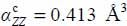 and
and 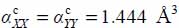 .
.
6.1.3. Graphite substrate–molecule interaction energy
The interaction potential energy VMS between the molecule and the substrate is the sum of the contributions of, by molecule–graphite atom (Gr) pairs, the Lennard-Jones dispersion–repulsion VLJ, the induction VI and the electrostatic VE.
6.1.3.1. Dispersion–repulsion contribution
In order to take into account the above-mentioned anisotropy phenomenon, Carlos and Cole [CAR 80] proposed a modified form of the atom–atom potential energy:
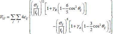
where γR and γA are coefficients associated with the anisotropy and θij is the angle between the axis  and the vector
  linking the atom i of the molecule and the graphite atom j, which can be written as:

that is, as a function of the position vectors of the carbon atom j and the center of mass of the molecule in the fixed reference frame, and the position vector of atom i of the molecule in the coordinate system linked to the latter. This vector then contains the dependency in terms of internal vibrational and orientational coordinates of the molecule.
The values of the atom–atom parameters of expression [6.3] are presented in Table 6.1.
Table 6.1. Lennard-Jones atom–atom parameters and atom–atom parameters associated with anisotropy of graphite carbon atoms (Gr)
| Atom– Gr | ε (cm−1) | σ (Å) | γA | γR |
| C–Gr | 24.04 | 3.305 | 0.4 | –1.05 |
| O–Gr | 27.82 | 3.141 | 0.4 | –1.05 |
| N–Gr | 22.67 | 3.390 | 0.4 | –1.05 |
| H–Gr | 18.30 | 2.965 | 0.4 | –0.54 |
6.1.3.2. Electrostatic and induction contributions
These contributions were introduced in Chapter 4 of Volume 1 [DAH 17]. They describe the interaction between the permanent multipolar moments of the molecule–graphite carbon atom partners and the interaction between these permanent moments and the electric field they create at the position of each partner:

The geometric and electrical characteristics of the HCN and H2O molecules are presented in Table 6.2.
Table 6.2. Characteristics of HCN and H2O molecules: geometric (bond length and angle between them), dipole moment, polarizability, quadrupole moment and rotational constants defined in the molecular coordinate system
| Molecule | HCN | H2O | ||
| Bond length (Å) | H-C | 1.079 | O-H | 0.958 |
| C-N | 1.150 | |||
| Angle between bonds (°) | 180 | 109.4 | ||
 |
2.986 | 1.855 | ||
| αxx(Å3) | 2.05 | 1.53 | ||
| αyy(Å3) | 2.05 | 1.42 | ||
| αzz(Å3) | 3.66 | 1.47 | ||
| Θxx(DÅ) | −2.20 | 2.63 | ||
| Θyy(DÅ) | −2.20 | −2.50 | ||
| Θzz(DÅ) | 4.40 | −0.13 | ||
| A (cm−1) | 1.48 | 27.33 | ||
| B (cm−1) | 1.48 | 14.57 | ||
| C (cm−1) | - | 9.49 | ||
6.2. Adsorption observables at low temperature
6.2.1. Equilibrium configuration and potential energy surface
The substrate used in our study is a crystal consisting of 10 planes each with a radius of 35 Å, to avoid edge effects that the molecule can experience.
As the molecule and the substrate are assumed to be rigid, two observables characterizing the adsorption can be determined: the adsorption energy and the diffusion constant of the molecule on the surface of the substrate.
The potential energy surface VMS(X0, Y0) of the lateral movement of the molecule is determined by minimizing  with respect to the approach distance Z0 (distance between the molecule’s center of mass and the surface) and the angular coordinates(φ0, θ0, χ0).
6.2.1.1. HCN molecule
The equilibrium configuration and site of the molecule are associated with the minimum energy value:
 for a position characterized by
  ,
,  and
and  and an orientation characterized by
  and
and  , the molecule being almost flat, above the middle of the C–C bond of the graphite with the hydrogen atom pointing towards the center of the hexagon (Figure 6.3).
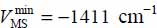
On the contrary, the maximum energy value is  obtained for an approach distance of Z0 = 3.24 Å, the molecule being almost flat above the surface and close to the center of the hexagon.
The potential energy surface VMS(X0, Y0) is shown in Figure 6.3. The diffusion path between two adjacent equilibrium configurations is also indicated. The diffusion energy barrier is 104 cm–1.

Figure 6.3. Potential energy surface VMS(X0,Y0) of the HCN molecule in its lateral movement above a graphite cell (left) and diffusion pathways on the surface (right). For a color version of this figure, see www.iste.co.uk/dahoo/infrared2.zip
6.2.1.2. H2O molecule
In the case of the H2O molecule, the minimum energy and the equilibrium configuration of the molecule are:
 for a position characterized by
  ,
,  and
and  and an orientation characterized by
  ,
,  and
and  , the molecule being almost flat (its plane is almost parallel to the surface), close to a carbon atom and straddling the C–C bond (Figure 6.4).
On the contrary, the maximum value  is obtained for an approach distance of Z0= 2.92 Å above the center of the hexagon
  , its C2 symmetry axis being perpendicular to the surface with the hydrogen atoms pointing upwards.
The potential energy surface VMS(X0, Y0) is shown in Figure 6.4. The diffusion path between two adjacent equilibrium configurations is also indicated. The diffusion energy barrier is 10 cm舑1. The molecule can therefore move almost freely on the surface.

Figure 6.4. Potential energy surface VMS(X0, Y0) of the molecule H2O in its lateral movement over a graphite cell (left) and diffusion paths on the surface (right). For a color version of this figure, see www.iste.co.uk/dahoo/infrared2.zip
6.2.2. Adsorption energy
The adsorption energy Ea of an adsorbed molecule on a surface at a temperature T is defined as the energy required to keep this molecule, with thermal energy  , at its equilibrium configuration on this surface. It is approximately given by:
where n is the number of external degrees of freedom of the molecule (6 for a nonlinear molecule and 5 for a diatomic or linear molecule) and ωs (s = 1 at n) are the frequencies associated with the translational and orientational movements of the molecule around its equilibrium configuration. These frequencies are determined by solving the Schrödinger equation associated with each movement using the “Discrete Variable Representation” method [LIG 85].
The values obtained for the frequencies ωs and adsorption energy Ea as a function of temperature are presented in Table 6.3.
Table 6.3. Frequencies (in cm–1) of the translational and orientational movements of HCN and H2O adsorbed on the graphite surface and their adsorption energy (in cm–1) as a function of temperature
| ωx | ωY | ωz | ωθ | ωφ | ωχ | Ea(10K) | Ea(40K) | Ea(100K) | |
| HCN | 21.0 | 23.4 | 79.0 | 109.7 | 32.3 | – | 1,363 | 1,323 | 1,290 |
| H2O | ~0 | ~0 | 90.3 | 35.5 | 22.6 | 233.9 | 952 | 1,000 | 1,048 |
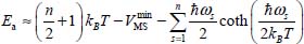
6.2.3. Diffusion constant
Let ∆VMS(τ) be the potential energy variation along the diffusion path between two adjacent equilibrium sites of respective positions τ1 and τ2, as shown in Figure 6.5. The set of diffusion coordinate values τ is in fact the set of coordinate points (X0, Y0) relative to the fixed reference frame.

Figure 6.5. Diffusion path between two equilibrium sites. In the case of HCN and H2O on the graphite surface, both sites are equivalent
Using the classical transition theory between states [VOT 84], the hopping frequency through the maximum energy position τ0 is defined by:
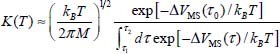
where M is the mass of the molecule and ΔVMS (τ0) is the value of the energy at the maximum of the diffusion path. The diffusion constant is therefore:
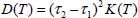
Table 6.4 presents the values of the distance between the two adjacent equilibrium sites, the height of the energy barrier and the diffusion constants at different temperatures.
Table 6.4. Diffusion characteristics of HCN and H2O on the graphite surface. Distance between the two equilibrium sites: height of the diffusion barrier and diffusion constants
| (τ2 – τ1) (Å) | Δ VMS(τ0) (cm舑1) | D (10K) (cm2/s) | D (40K) (cm2/s) | D (100K) (cm2/s) | |
| HCN | 2.46 | 104 | 1.1 × 10⁻¹⁰ | 1.2 × 10⁻⁵ | 7.2 × 10⁻⁵ |
| H2O | 1.02 | 10 | 1.5 × 10⁻⁵ | 4.3 × 10⁻⁵ | 7.2 × 10⁻⁵ |
It is found that at the temperature T = 10 K, the H2O molecule can diffuse five times more easily than the HCN molecule. This is due, on the one hand, to the difference in energy barriers to be crossed, and, on the other hand, to the mass difference in the two molecules. Whereas when the temperature increases, the diffusion constants of both molecules tend to be of the same order of magnitude.
6.3. Interaction energy between two molecules
A possible clustering of the HCN, H2O, H2CO and NH3, molecules, previously and randomly adsorbed on a graphite substrate simulating an interstellar dust grain, which would lead to the formation of a glycine molecule (Figure 6.1), requires a detailed study of the interactions between these different partners (molecules and substrate). It is a tedious task that can only be done numerically. Therefore, we will develop the long-range contributions, electrostatic and induction interaction, at a relatively high multipolar order, which is included in the computation program.
In the approximation of binary interactions, we must calculate at each time the “molecule–molecule”, “molecule–surface” interaction energies. The latter was presented in section 6.1.3.
In order to determine the “molecule–molecule” interaction energy, we consider two molecules at position vectors  and
and  relative to a fixed (absolute) reference frame
  , as shown in Figure 6.6. These two molecules are each tied to a mobile reference frame
  and are electrically characterized by their charge distributions, their permanent multipolar moments (dipole
  , quadrupole
  , octupole
  , etc.) and their dipole polarizability
  .
.

Figure 6.6 Interaction between two molecules with respect to a fixed reference (absolute) frame  . Example HCN and H2O. For a color version of this figure, see www.iste.couk/dahoo/infrared2.zip
6.3.1. Electrostatic contribution
This contribution is due to the interaction between the permanent multipole moments of the two electrically neutral molecules. However, depending on the distance between the two molecules, they can interact through their charge distributions or through their permanent multipole moments.
Indeed, if the distance is around the size of the molecules, the electrostatic energy is written as:

where qi and qj are respectively the charge of site i of molecule 1 and the charge of site j of molecule 2, and  is the distance vector between these two sites. Note that, depending on the molecule, the sites carrying the charges may be different from the atoms constituting this molecule.
However, when the distance between the two molecules is large enough with respect to their size, each appears neutral to the other, and they interact via their multipolar moments.
Each molecule creates an electric potential in its surrounding space. Let Φ1→2 and Φ2→1 be the electrical potentials created, respectively, by molecule 1 at position  and by molecule 2 at position
  (Figure 6.6), they are defined by [BUC 67]:


where  is the distance vector between the two molecules (between the centers of mass), of components relative to the fixed reference frame R12α = R2α - R1α (α = X,Y,Z);
  are their dipole (vector), quadrupole (rank-2 tensor), octupole (rank-3 tensor) moments …, also expressed with respect to the fixed reference frame (Appendix 6.4.2); and ε0 is the electrical permittivity of the vacuum.
In the expressions [6.11a] and [6.11b], the symbol  designates the gradient operator which acting on a function f (X,Y,Z), results in the vector:

The electrostatic interaction potential energy between the two molecules is defined as [BUC 67]:

or

By putting the expression [6.11a] (or [6.11b]) in expression [6.13b] (or [6.13a]), we obtain:

which we write, by introducing the components with respect to the fixed reference of the different vectors and tensors, as:
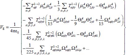
where  are called the rank-2 “action tensor” for
  , rank-3 action tensor for
  and rank n action tensor for
  ; their expressions are given in Appendix 6.4.1. The indices α, β,... (α = X, Y, Z , β = X,Y,Z, …) represent the directions of the axes of the frame.
Moreover, since the distance vector is given by  , the action tensors verify the property
  .
.
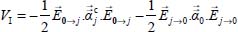
6.3.2. Induction contribution
As we mentioned before, with the molecules being polarizable, each one creates induced multipolar moments on the other. The induction potential energy is due to the interaction between the induced moments and the permanent moments. It is defined by:

where  are the electric fields created by each of the two molecules on the other; they are defined as:

and  are the dipolar polarizabilities (rank-2 tensors) of the partner molecules, defined with respect to the fixed reference frame (Appendix 6.4.2).
By introducing the components of the different vectors and tensors, the expression [6.16] is written as:

with

and

6.3.3. Dispersion–repulsion contribution
This part is generally modeled by a Lennard-Jones atom–atom potential energy in the form:
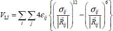
where  is the distance vector between atom i of molecule 1 and atom j of molecule 2, as shown in Figure 6.6.
On the one hand, the first term of this expression (in 1/R12) is a repulsion term, dominant at short-range, which arises from the overlap of the electronic clouds of the two atoms. The second term (in 1/R6) is attractive, dominant at long-range, and is due to the interaction between multipoles induced on the two atoms.
On the other hand, the Lennard-Jones potential parameters εij and σij are defined by the equations  and
and  (Figure 4.2, Chapter 4 of Volume 1 [DAH 17]). They are determined by the combination rules of Lorentz–Berthelot

Finally, to help the reader to calculate the three contributions to the interaction potential energy between any two molecules, a program in the FORTRAN language is presented in Appendix 6.4.3. This program can easily be translated into another language.
6.4. Appendices
6.4.1. Expressions of action tensors
To simplify the following expressions,  and its components R12α are replaced, respectively, by
  and Rα:


6.4.2. Multipolar moments and dipolar polarizability of a molecule relative to the fixed (absolute) reference frame

where M-1 (φ, θ, χ) is the inverse matrix of the unitary rotational matrix transformation M(φ, θ, χ) (Appendix 2.7.1 in Chapter 2) associated with the molecule (1 or 2). In these expressions, the multipole moments  , and the dipole polarizability
  , are defined relative to the mobile reference frame
  linked to the molecule.
6.4.3. Code in the FORTRAN language for the calculation of the interaction potential energy between two molecules
C*****************************************************************
C* Calculation of Interaction Potential Energy
C* Between Two Molecules : For example HCN - H2CO (Formaldehyde)
C*                                       1 - 2
C*****************************************************************
C* 1 ----> Atom N     1 --> Atom O
C* 2 ---->      C     2 ---->    C
C* 3 ---->      H     3 ---->    side H x positive
C*                    4 ---->    side H x negative
C*****************************************************************
   IMPLICIT DOUBLE PRECISION (A-H,O-Z)
   DIMENSION RM12(3)   ! Vector distance mol 1---mol 2
   DIMENSION HX1(3),HY1(3),HZ1(3),DM1(3,3),OCT1(3,3,3)
   DIMENSION DIPM1(3),ALM1(3,3),QUM1(3,3),OCTUM1(3,3,3)
   DIMENSION HX2(4),HY2(4),HZ2(4),DM2(3,3),OCT2(3,3,3)
   DIMENSION DIPM2(3),ALM2(3,3),QUM2(3,3),OCTUM2(3,3,3)
   DIMENSION ECM12(3),ECMDIP12(3),ECMQUA12(3),ECMOCT12(3)
   DIMENSION ECM21(3),ECMDIP21(3),ECMQUA21(3),ECMOCT21(3)
   DIMENSION C6(3,4),C12(3,4)
C*****************************************************************
C* Definition Of Some Values
C*****************************************************************
   PI= DACOS(-1.D0)
   S2= DSQRT(2.D0)
   S3= DSQRT(3.D0)
   ABOHR= 0.52917725D0    ! Bohr Radius
   UAMEV= 27211.4D0      ! Conversion factor of energy u.a. → meV
C*****************************************************************
C* Lennard-Jones Parameters in u.a.
C* C6 ET C12 (Atom Of Molecule 1 – Atom Of Molecule 2)
C* C6 = 4 x epsilon x sigma**6
C* C12 = 4 x epsilon x sigma**12
C*****************************************************************
   C6(1,1)= 122548.8D0 / 4820.167394D0    ! N - O
   C6(1,2)= 143846.3D0 / 4820.167394D0    ! N - C
   C6(1,3)= 56859.5D0 / 4820.167394D0     ! N - H
   C6(1,4)= 56859.5D0 / 4820.167394D0     ! N - H
   C12(1,1)= 115453563.D0 / 105.832398D0
   C12(1,2)= 184090484.D0 / 105.832394D0
   C12(1,3)= 37857130.D0 / 105.832394D0
   C12(1,4)= 37857130.D0 / 105.832394D0
C***************************************************
   C6(2,1)= 110155.6D0 / 4820.167394D0     ! C - O
   C6(2,2)= 130408.7D0 / 4820.167394D0     ! C - C
   C6(2,3)= 50609.0D0 / 4820.167394D0      ! C - H
   C6(2,4)= 50609.0D0 / 4820.167394D0      ! C - H
   C12(2,1)= 87980421.D0 / 105.832398D0
   C12(2,2)= 142671308.D0 / 105.832394D0
   C12(2,3)= 28282590.D0 / 105.832394D0
   C12(2,4)= 28282590.D0 / 105.832394D0
C***************************************************
   C6(3,1)= 41146.0D0 / 4820.167394D0     ! H - O
   C6(3,2)= 50609.0D0 / 4820.167394D0     ! H - C
   C6(3,3)= 18043.1D0 / 4820.167394D0     ! H - H
   C6(3,4)= 18043.1D0 / 4820.167394D0     ! H - H
   C12(3,1)= 16154547.D0 / 105.832398D0
   C12(3,2)= 28282590.D0 / 105.832394D0
   C12(3,3)= 4731890.D0 / 105.832394D0
   C12(3,4)= 4731890.D0 / 105.832394D0
C*****************************************************************
C
C Characteristics of molecule 1       HCN
C
C*****************************************************************
C* Geometric And Electric Parameters IN u.a.
C*****************************************************************
C* Dipolar Polarizability, Dipole, Quadupole and Octupole moments
C* in the mobile reference frame of the molecule
C* Note. For polarizability, dipole and quadrupole moments, only
C*      non-zero components appear!
C*****************************************************************
   AL1xx= 13.834D0
   AL1yy= 13.834D0
   AL1zz= 24.700D0
   DIP1= 1.17486D0
   QUA1xx= -1.635755D0
   QUA1yy= -1.635755D0
   QUA1zz= 3.271510D0
   OCT1(1,1,1)= 0.
   OCT1(1,1,2)= 0.
   OCT1(1,1,3)= 0.
   OCT1(1,2,1)= 0.
   OCT1(1,2,2)= 0.
   OCT1(1,2,3)= 0.
   OCT1(1,3,1)= 0.
   OCT1(1,3,2)= 0.
   OCT1(1,3,3)= 0.
   OCT1(2,1,1)= 0.
   OCT1(2,1,2)= 0.
   OCT1(2,1,3)= 0.
   OCT1(2,2,1)= 0.
   OCT1(2,2,2)= 0.
   OCT1(2,2,3)= 0.
   OCT1(2,3,1)= 0.
   OCT1(2,3,2)= 0.
   OCT1(2,3,3)= 0.
   OCT1(3,1,1)= 0.
   OCT1(3,1,2)= 0.
   OCT1(3,1,3)= 0.
   OCT1(3,2,1)= 0.
   OCT1(3,2,2)= 0.
   OCT1(3,2,3)= 0.
   OCT1(3,3,1)= 0.
   OCT1(3,3,2)= 0.
   OCT1(3,3,3)= 0.
C*****************************************************************
C* Positions Of Atoms In The Molecule Reference Frame
C*****************************************************************
   HX1(1)= 0.D0
   HY1(1)= 0.D0
   HZ1(1)= -0.5943D0/ABOHR
   HX1(2)= 0.D0
   HY1(2)= 0.D0
   HZ1(2)= 0.5559D0/ABOHR
   HX1(3)= 0.D0
   HY1(3)= 0.D0
   HZ1(3)= 1.6349D0/ABOHR
C*****************************************************************
C* Position Of The Center Of Mass In u.a. And Orientation Of The Molecule
C*****************************************************************
   X01=0.D0
   Y01=0.D0
   Z01=0.D0
   PHI01=0.D0
   TE01=0.D0
   QUI01=0.D0
   XM1= X01/ABOHR
   YM1= Y01/ABOHR
   ZM1= Z01/ABOHR
C*****************************************************************
   PHI1= PHI01*PI/180.D0
   SA1=DSIN(PHI1)
   CA1=DCOS(PHI1)
C*****************************************************************
   TE1= TE01*PI/180.D0
   SB1=DSIN(TE1)
   CB1=DCOS(TE1)
C*****************************************************************
   QUI1= QUI01*PI/180.D0
   SC1=DSIN(QUI1)
   CC1=DCOS(QUI1)
C*****************************************************************
C* Inverse Matrix M-1 Of Unitary Transformation
C*****************************************************************
   RM1Xx= CA1*CB1*CC1 - SA1*SC1
   RM1Xy=-CA1*CB1*SC1 - SA1*CC1
   RM1Xz= CA1*SB1
   RM1Yx= SA1*CB1*CC1 + CA1*SC1
   RM1Yy=-SA1*CB1*SC1 + CA1*CC1
   RM1Yz= SA1*SB1
   RM1Zx=-SB1*CC1
   RM1Zy= SB1*SC1
   RM1Zz= CB1
C
   DM1(1,1)= RM1Xx
   DM1(1,2)= RM1Xy
   DM1(1,3)= RM1Xz
   DM1(2,1)= RM1Yx
   DM1(2,2)= RM1Yy
   DM1(2,3)= RM1Yz
   DM1(3,1)= RM1Zx
   DM1(3,2)= RM1Zy
   DM1(3,3)= RM1Zz
C*****************************************************************
C* Components In The Absolute Reference Frame Of Tensors: Polarizability,
C* Dipole Moment, Quadrupole Moment, Octupole Moment
C* Of Molecule 1
C*****************************************************************
   ALM1(1,1)= RM1Xx*RM1Xx*AL1xx+RM1Xy*RM1Xy*AL1yy+
   &          RM1Xz*RM1Xz*AL1zz
   ALM1(1,2)= RM1Xx*RM1Yx*AL1xx+RM1Xy*RM1Yy*AL1yy+
   &          RM1Xz*RM1Yz*AL1zz
   ALM1(1,3)= RM1Xx*RM1Zx*AL1xx+RM1Xy*RM1Zy*AL1yy+
   &          RM1Xz*RM1Zz*AL1zz
   ALM1(2,1)= ALM1(1,2)
   ALM1(2,2)= RM1Yx*RM1Yx*AL1xx+RM1Yy*RM1Yy*AL1yy+
   &          RM1Yz*RM1Yz*AL1zz
   ALM1(2,3)= RM1Yx*RM1Zx*AL1xx+RM1Yy*RM1Zy*AL1yy+
   &          RM1Yz*RM1Zz*AL1zz
   ALM1(3,1)= ALM1(1,3)
   ALM1(3,2)= ALM1(2,3)
   ALM1(3,3)= RM1Zx*RM1Zx*AL1xx+RM1Zy*RM1Zy*AL1yy+
   &          RM1Zz*RM1Zz*AL1zz
C*****************************************************************
   DIPM1(1) = DIP1*RM1Xz
   DIPM1(2) = DIP1*RM1Yz
   DIPM1(3) = DIP1*RM1Zz
C*****************************************************************
   QUM1(1,1)= RM1Xx*RM1Xx*QUA1xx+RM1Xy*RM1Xy*QUA1yy
   &          +RM1Xz*RM1Xz*QUA1zz
   QUM1(1,2)= RM1Xx*RM1Yx*QUA1xx+RM1Xy*RM1Yy*QUA1yy
   &          +RM1Xz*RM1Yz*QUA1zz
   QUM1(1,3)= RM1Xx*RM1Zx*QUA1xx+RM1Xy*RM1Zy*QUA1yy
   &          +RM1Xz*RM1Zz*QUA1zz
   QUM1(2,1)= QUM1(1,2)
   QUM1(2,2)= RM1Yx*RM1Yx*QUA1xx+RM1Yy*RM1Yy*QUA1yy
   &          +RM1Yz*RM1Yz*QUA1zz
   QUM1(2,3)= RM1Yx*RM1Zx*QUA1xx+RM1Yy*RM1Zy*QUA1yy
   &          +RM1Yz*RM1Zz*QUA1zz
   QUM1(3,1)= QUM1(1,3)
   QUM1(3,2)= QUM1(2,3)
   QUM1(3,3)= RM1Zx*RM1Zx*QUA1xx+RM1Zy*RM1Zy*QUA1yy
   &          +RM1Zz*RM1Zz*QUA1zz
C*****************************************************************
   DO 111 I=1,3
   DO 112 J=1,3
   DO 113 k=1,3
   DO 114 II=1,3
   DO 115 JJ=1,3
   DO 116 KK=1,3
   OCTUM1(I,J,K)= OCTUM1(I,J,K)
   & + DM1(I,II) * DM1(J,JJ) * DM1(K,KK) * OCT1(II,JJ,KK)
116 CONTINUE
115 CONTINUE
114 CONTINUE
113 CONTINUE
112 CONTINUE
111 CONTINUE
C*****************************************************************
C
C Characteristics of molecule 2       H2CO
C
C*****************************************************************
C* Geometric And Electric Parameters In u.a.
C*****************************************************************
C* Dipole Polarizability, Dipole, Quadrupole And Octupole Moments
C* in the mobile reference frame of the molecule
C* Note. For polarizability, dipole and quadrupole moments, only
C*        non-zero components appear!
C*****************************************************************
   AL2xx= 16.938D0
   AL2yy= 13.092D0
   AL2zz= 19.570D0
   DIP2= 0.91675D0
   QUA2xx= 1.42162D0
   QUA2yy= -3.72134D0
   QUA2zz= 2.29972D0
   OCT2(1,1,1)= 0.
   OCT2(1,1,2)= 0.
   OCT2(1,1,3)= 0.
   OCT2(1,2,1)= 0.
   OCT2(1,2,2)= 0.
   OCT2(1,2,3)= 0.
   OCT2(1,3,1)= 0.
   OCT2(1,3,2)= 0.
   OCT2(1,3,3)= 0.
   OCT2(2,1,1)= 0.
   OCT2(2,1,2)= 0.
   OCT2(2,1,3)= 0.
   OCT2(2,2,1)= 0.
   OCT2(2,2,2)= 0.
   OCT2(2,2,3)= 0.
   OCT2(2,3,1)= 0.
   OCT2(2,3,2)= 0.
   OCT2(2,3,3)= 0.
   OCT2(3,1,1)= 0.
   OCT2(3,1,2)= 0.
   OCT2(3,1,3)= 0.
   OCT2(3,2,1)= 0.
   OCT2(3,2,2)= 0.
   OCT2(3,2,3)= 0.
   OCT2(3,3,1)= 0.
   OCT2(3,3,2)= 0.
   OCT2(3,3,3)= 0.
C*****************************************************************
C* Positions Of Atoms In The Mobile Reference Frame Of The Molecule
C******************************************************************
   HX2(1)= 0.D0
   HY2(1)= 0.D0
   HZ2(1)= -0.5994D0/ABOHR
   HX2(2)= 0.D0
   HY2(2)= 0.D0
   HZ2(2)= 0.5986D0/ABOHR
   HX2(3)= 0.9520D0/ABOHR
   HY2(3)= 0.D0
   HZ2(3)= 1.1911D0/ABOHR
   HX2(4)= -0.9520D0/ABOHR
   HY2(4)= 0.D0
   HZ2(4)= 1.1911D0/ABOHR
C*****************************************************************
C* Position Of Center Of Mass In u.a. And Orientation Of The Molecule
C*****************************************************************
   DO 60 IX2= 1,11
   X02= 3.D0 + (IX2-1)*0.1D0   ! Ang
   WRITE(*,11)X02
11 FORMAT(///5X,F7.1)
   Y02=0.D0
   Z02=0.D0
   XM2= X02/ABOHR
   YM2= Y02/ABOHR
   ZM2= Z02/ABOHR
C*****************************************************************
   PHI02=0.D0
   PHI2= PHI02*PI/180.D0
   SA2=DSIN(PHI2)
   CA2=DCOS(PHI2)
C*****************************************************************
   DO 70 IT2= 1,19
   TE02= (IT2-1)*10.D0
   TE2= TE02*PI/180.D0
   SB2=DSIN(TE2)
   CB2=DCOS(TE2)
C*****************************************************************
   QUI02=0.D0
   QUI2= QUI02*PI/180.D0
   SC2=DSIN(QUI2)
   CC2=DCOS(QUI2)
C*****************************************************************
C* Inverse Matrix M-1 Of Unitary Transformation
C*****************************************************************
   RM2Xx= CA2*CB2*CC2 - SA2*SC2
   RM2Xy=-CA2*CB2*SC2 - SA2*CC2
   RM2Xz= CA2*SB2
   RM2Yx= SA2*CB2*CC2 + CA2*SC2
   RM2Yy=-SA2*CB2*SC2 + CA2*CC2
   RM2Yz= SA2*SB2
   RM2Zx=-SB2*CC2
   RM2Zy= SB2*SC2
   RM2Zz= CB2
C
   DM2(1,1)= RM2Xx
   DM2(1,2)= RM2Xy
   DM2(1,3)= RM2Xz
   DM2(2,1)= RM2Yx
   DM2(2,2)= RM2Yy
   DM2(2,3)= RM2Yz
   DM2(3,1)= RM2Zx
   DM2(3,2)= RM2Zy
   DM2(3,3)= RM2Zz
C*****************************************************************
C* Components In The Absolute Reference Frame Of Tensors: Polarizability,
C* Dipole Moment, Quadrupole Moment, Octupole Moment
C* Of Molecule 2
C*****************************************************************
   ALM2(1,1)= RM2Xx*RM2Xx*AL2xx+RM2Xy*RM2Xy*AL2yy+
   &          RM2Xz*RM2Xz*AL2zz
   ALM2(1,2)= RM2Xx*RM2Yx*AL2xx+RM2Xy*RM2Yy*AL2yy+
   &          RM2Xz*RM2Yz*AL2zz
   ALM2(1,3)= RM2Xx*RM2Zx*AL2xx+RM2Xy*RM2Zy*AL2yy+
   &          RM2Xz*RM2Zz*AL2zz
   ALM2(2,1)= ALM2(1,2)
   ALM2(2,2)= RM2Yx*RM2Yx*AL2xx+RM2Yy*RM2Yy*AL2yy+
   &          RM2Yz*RM2Yz*AL2zz
   ALM2(2,3)= RM2Yx*RM2Zx*AL2xx+RM2Yy*RM2Zy*AL2yy+
   &          RM2Yz*RM2Zz*AL2zz
   ALM2(3,1)= ALM2(1,3)
   ALM2(3,2)= ALM2(2,3)
   ALM2(3,3)= RM2Zx*RM2Zx*AL2xx+RM2Zy*RM2Zy*AL2yy+
   &          RM2Zz*RM2Zz*AL2zz
C*****************************************************************
   DIPM2(1) = DIP2*RM2Xz
   DIPM2(2) = DIP2*RM2Yz
   DIPM2(3) = DIP2*RM2Zz
C*****************************************************************
   QUM2(1,1)= RM2Xx*RM2Xx*QUA2xx+RM2Xy*RM2Xy*QUA2yy
   &                +RM2Xz*RM2Xz*QUA2zz
   QUM2(1,2)= RM2Xx*RM2Yx*QUA2xx+RM2Xy*RM2Yy*QUA2yy
   &                +RM2Xz*RM2Yz*QUA2zz
   QUM2(1,3)= RM2Xx*RM2Zx*QUA2xx+RM2Xy*RM2Zy*QUA2yy
   &                +RM2Xz*RM2Zz*QUA2zz
   QUM2(2,1)= QUM2(1,2)
   QUM2(2,2)= RM2Yx*RM2Yx*QUA2xx+RM2Yy*RM2Yy*QUA2yy
   &                +RM2Yz*RM2Yz*QUA2zz
   QUM2(2,3)= RM2Yx*RM2Zx*QUA2xx+RM2Yy*RM2Zy*QUA2yy
   &                +RM2Yz*RM2Zz*QUA2zz
   QUM2(3,1)= QUM2(1,3)
   QUM2(3,2)= QUM2(2,3)
   QUM2(3,3)= RM2Zx*RM2Zx*QUA2xx+RM2Zy*RM2Zy*QUA2yy
   &                +RM2Zz*RM2Zz*QUA2zz
C*****************************************************************
   DO 221 I=1,3
   DO 222 J=1,3
   DO 223 k=1,3
   DO 224 II=1,3
   DO 225 JJ=1,3
   DO 226 KK=1,3
   OCTUM2(I,J,K)= OCTUM2(I,J,K)
   & + DM2(I,II) * DM2(J,JJ) * DM2(K,KK) * OCT2(II,JJ,KK)
226 CONTINUE
225 CONTINUE
224 CONTINUE
223 CONTINUE
222 CONTINUE
221 CONTINUE
C*****************************************************************
C
C   Calculation C
C*****************************************************************
C* Calculation Of Different Contributions
C* VEDIP1DIP2 ==> ELECT DIP MOL1 - DIP MOL2
C* VEDIP1QUA2 ==> ELECT DIP MOL1 - QUAD MOL2
C* VEDIP1OCT2 ==> ELECT DIP MOL1 - OCTUP MOL2
C* VEQUA1DIP2 ==> ELECT QUAD MOL1 - DIP MOL2
C* VEQUA1QUA2 ==> ELECT QUAD MOL1 - QUAD MOL2
C* VEQUA1OCT2 ==> ELECT QUAD MOL1 - OCTUP MOL2
C* VEOCT1DIP2 ==> ELECT OCTUP MOL1 - DIP MOL2
C* VEOCT1QUA2 ==> ELECT OCTUP MOL1 - QUAD MOL2
C* VEOCT1OCT2 ==> ELECT OCTUP MOL1 - OCTUP MOL2
C* VIM12 ==> INDUC MOL1 ---> MOL2
C* VIM21 ==> INDUC MOL2 ---> MOL1
C* VLJ12 ==> Lennard-Jones (Dispersion-Repulsion)
C*****************************************************************
C* Reset to Zero
C*****************************************************************
   VEDIP1DIP2= 0.D0
   VEDIP1QUA2= 0.D0
   VEDIP1OCT2= 0.D0
   VEQUA1DIP2= 0.D0
   VEQUA1QUA2= 0.D0
   VEQUA1OCT2= 0.D0
   VEOCT1DIP2= 0.D0
   VEOCT1QUA2= 0.D0
   VEOCT1OCT2= 0.D0
   VIM12= 0.D0
   VIM21= 0.D0
   VLJ12= 0.D0
C*****************************************************************
C* Vector Components of Distance Mol1 - Mol2 in u.a.
C*****************************************************************
   RM12(1)= XM2 - XM1
   RM12(2)= YM2 - YM1
   RM12(3)= ZM2 - ZM1
C*****************************************************************
   RM2= RM12(1)**2+RM12(2)**2+RM12(3)**2
   RM1= DSQRT(RM2)
   RM4= RM2*RM2
   RM5= RM4*RM1
   RM7= RM5*RM2
   RM9= RM7*RM2
   RM11= RM9*RM2
   RM13= RM11*RM2
C*****************************************************************
C* Calculation of Electrostatic and Indiuction Contributions
C*****************************************************************
C* Reset Electric Field Induced By Molecule 1 (2)
C* On Position Of Molecule 2 (1)
C*      ECM12 = ECMDIP12 + ECMQUA12 + ECMOCT12
C*      ECM21 = ECMDIP21 + ECMQUA21 + ECMOCT21
C*****************************************************************
   DO 30 I=1,3
   ECMDIP12(I)= 0.D0
   ECMQUA12(I)= 0.D0
   ECMOCT12(I)= 0.D0
   ECMDIP21(I)= 0.D0
   ECMQUA21(I)= 0.D0
   ECMOCT21(I)= 0.D0
30 CONTINUE
C*****************************************************************
   DO 31 I1=1,3
   DO 32 I2=1,3
   TACTION2= TAC2(I1,I2,RM12,RM2,RM5) ! Rank-2 Action Tensor
   ECMDIP12(I1)= ECMDIP12(I1) + TACTION2 * DIPM1(I2)
   ECMDIP21(I1)= ECMDIP21(I1) + TACTION2 * DIPM2(I2)
   VEDIP1DIP2= VEDIP1DIP2 - DIPM1(I1)*TACTION2 * DIPM2(I2)
   DO 33 I3=1,3
   TACTION3= TAC3(I1,I2,I3,RM12,RM2,RM7) ! Rank-3 Action Tensor
   ECMQUA12(I1)= ECMQUA12(I1) - TACTION3 * QUM1(I2,I3)/3.D0
   ECMQUA21(I1)= ECMQUA21(I1) + TACTION3 * QUM2(I2,I3)/3.D0
   VEDIP1QUA2= VEDIP1QUA2 - DIPM1(I1)* TACTION3 *QUM2(I2,I3)/3.D0
   VEQUA1DIP2= VEQUA1DIP2 + QUM1(I1,I2)*TACTION3*DIPM2(I3)/3.D0
   DO 34 I4=1,3
   TACTION4= TAC4(I1,I2,I3,I4,RM12,RM2,RM4,RM9) ! Rank-4 Action Tensor
   ECMOCT12(I1)= ECMOCT12(I1) + TACTION4 * OCTUM1(I2,I3,I4)/15.D0
   ECMOCT21(I1)= ECMOCT21(I1) + TACTION4 * OCTUM2(I2,I3,I4)/15.D0
   VEDIP1OCT2= VEDIP1OCT2 - DIPM1(I1) * TACTION4
   &              * OCTUM2(I2,I3,I4)/15.D0
   VEQUA1QUA2= VEQUA1QUA2 + QUM1(I1,I2) * TACTION4
   &              * QUM2(I3,I4)/9.D0
   VEOCT1DIP2= VEOCT1DIP2 - OCTUM1(I1,I2,I3) * TACTION4
   &              * DIPM2(I4)/15.D0
   DO 35 I5=1,3
   TACTION5= TAC5(I1,I2,I3,I4,I5,RM12,RM7,RM9,RM11)
   VEQUA1OCT2= VEQUA1OCT2 + QUM1(I1,I2) * TACTION5
   &              * OCTUM2(I3,I4,I5)/45.D0
   VEOCT1QUA2= VEOCT1QUA2 - OCTUM1(I1,I2,I3) * TACTION5
   &              * QUM2(I4,I5)/45.D0
   DO 36 I6=1,3
   TACTION6= TAC6(I1,I2,I3,I4,I5,I6,RM12,RM7,RM9,RM11,RM13)
   VEOCT1OCT2= VEOCT1OCT2 - OCTUM1(I1,I2,I3) * TACTION6
   &              * OCTUM2(I4,I5,I6)/225.D0
 36 CONTINUE
 35 CONTINUE
 34 CONTINUE
 33 CONTINUE
 32 CONTINUE
 31 CONTINUE
   DO 37 I=1,3
   ECM12(I)= ECMDIP12(I) + ECMQUA12(I) + ECMOCT12(I)
 37 ECM21(I)=ECMDIP21(I)+ECMQUA21(I)+ECMOCT21(I)
   DO 38 I1=1,3
   DO 39 I2=1,3
   VIM12= VIM12 - 0.5D0*ECM12(I1)*ALM2(I1,I2)*ECM12(I2)
   VIM21= VIM21 - 0.5D0*ECM21(I1)*ALM1(I1,I2)*ECM21(I2)
 39 CONTINUE
 38 CONTINUE
C*******************************************
C* Contribution of induction VIM Total
C*******************************************
VIM= VIM12 + VIM21
C*****************************************************************
C* Calculation of the Quantum Lennard-Jones (Atom-Atom) Contribution
C*****************************************************************
   DO 50 J1= 1,3
   XJ1= RM1Xx*HX1(J1) + RM1Xy*HY1(J1) + RM1Xz*HZ1(J1)
   YJ1= RM1Yx*HX1(J1) + RM1Yy*HY1(J1) + RM1Yz*HZ1(J1)
   ZJ1= RM1Zx*HX1(J1) + RM1Zy*HY1(J1) + RM1Zz*HZ1(J1)
   DO 40 J2= 1,4
   XJ2= RM2Xx*HX2(J2) + RM2Xy*HY2(J2) + RM2Xz*HZ2(J2)
   YJ2= RM2Yx*HX2(J2) + RM2Yy*HY2(J2) + RM2Yz*HZ2(J2)
   ZJ2= RM2Zx*HX2(J2) + RM2Zy*HY2(J2) + RM2Zz*HZ2(J2)
C*****************************************************************
   XJ1J2= RM12(1) + XJ2 - XJ1
   YJ1J2= RM12(2) + YJ2 - YJ1
   ZJ1J2= RM12(3) + ZJ2 - ZJ1
   R2J1J2= XJ1J2**2 + YJ1J2**2 + ZJ1J2**2
   VLJ12= VLJ12 + (C12(J1,J2)/R2J1J2**6) - (C6(J1,J2)/R2J1J2**3)
 40 CONTINUE
 50 CONTINUE
C*****************************************************************
C* Total Potential Energy * UAMEV  ------> in meV
C*****************************************************************
   POT= (VEDIP1DIP2 + VEDIP1QUA2 + VEDIP1OCT2
   &           + VEQUA1DIP2 + VEQUA1QUA2 + VEQUA1OCT2
   &       + VEOCT1DIP2 + VEOCT1QUA2 + VEOCT1OCT2
   &   + VIM12 + VIM21 + VLJ12) * UAMEV
   VEDIP1DIP2= VEDIP1DIP2 * UAMEV
   VEDIP1QUA2= VEDIP1QUA2 * UAMEV
   VEDIP1OCT2= VEDIP1OCT2 * UAMEV
   VEQUA1DIP2= VEQUA1DIP2 * UAMEV
   VEQUA1QUA2= VEQUA1QUA2 * UAMEV
   VEQUA1OCT2= VEQUA1OCT2 * UAMEV
   VEOCT1DIP2= VEOCT1DIP2 * UAMEV
   VEOCT1QUA2= VEOCT1QUA2 * UAMEV
   VEOCT1OCT2= VEOCT1OCT2 * UAMEV
   VIM12= VIM12 * UAMEV
   VIM21= VIM21 * UAMEV
   VLJ12= VLJ12 * UAMEV
C*****************************************************************
   WRITE(*,10)VEDIP1DIP2,VEDIP1QUA2,VEDIP1OCT2,VEQUA1DIP2
   WRITE(*,10)VEQUA1QUA2,VEQUA1OCT2,VEOCT1DIP2,VEOCT1QUA2
   WRITE(*,10)VEOCT1OCT2,VIM12,VIM21,VLJ12,POT
 70 CONTINUE
 60 CONTINUE
 10 FORMAT(/5(9X,F11.2))
   STOP
   END
C*****************************************************************
C*****************************************************************
C* Calculation of Action Tensor Components of orders 2,3,4,5,6
C*****************************************************************
C
   FUNCTION TAC2(I,J,R,R2,R5)
   IMPLICIT DOUBLE PRECISION (A-H,O-Z)
   DIMENSION R(3)
C
   TAC2= (3.D0*R(I)*R(J)-R2*KR(I,J))/R5
C
   RETURN
   END
C******************************************************************
C
   FUNCTION TAC3(I,J,K,R,R2,R7)
   IMPLICIT DOUBLE PRECISION (A-H,O-Z)
   DIMENSION R(3)
C
   TAC3= -(15.D0*R(I)*R(J)*R(K)-3.D0*R2*(R(I)*KR(J,K)
   &            +R(J)*KR(I,K)+R(K)*KR(I,J)))/R7
C
   RETURN
   END
C******************************************************************
C
   FUNCTION TAC4(I,J,K,L,R,R2,R4,R9)
   IMPLICIT DOUBLE PRECISION (A-H,O-Z)
   DIMENSION R(3) C
   TAC4= (105.D0*R(I)*R(J)*R(K)*R(L)-15.D0*R2*(R(I)*R(J)*KR(K,L)
   &  +R(I)*R(K)*KR(J,L)+R(I)*R(L)*KR(J,K)+R(J)*R(K)*KR(I,L)
   &  +R(J)*R(L)*KR(I,K)+R(K)*R(L)*KR(I,J))
   &  +3.D0*R4*(KR(I,J)*KR(K,L)+KR(I,K)*KR(J,L)+KR(I,L)*KR(J,K)))/R9
C
   RETURN
   END
C******************************************************************
C
   FUNCTION TAC5(I,J,K,L,M,R,R7,R9,R11)
   IMPLICIT DOUBLE PRECISION (A-H,O-Z)
   DIMENSION R(3)
C
   TAC5= -945.D0*R(I)*R(J)*R(K)*R(L)*R(M) / R11
   & + 105.D0 * (R(I)*R(J)*R(K)*KR(L,M) + R(I)*R(J)*R(L)*KR(K,M)
   & + R(I)*R(K)*R(L)*KR(J,M) + R(J)*R(K)*R(L)*KR(I,M)
   & + R(I)*R(J)*R(M)*KR(K,L) + R(I)*R(K)*R(M)*KR(J,L)
   & + R(I)*R(L)*R(M)*KR(J,K) + R(J)*R(K)*R(M)*KR(I,L)
   & + R(J)*R(L)*R(M)*KR(I,K) + R(K)*R(L)*R(M)*KR(I,J)) / R9
   & - 15.D0 * (R(I)*(KR(J,L)*KR(K,M) + KR(J,K)*KR(L,M)
   &                      + KR(J,M)*KR(K,L))
   &     + R(J)*(KR(I,M)*KR(K,L) + KR(K,M)*KR(I,L)
   &                      + KR(I,K)*KR(L,M))
   &     + R(K)*(KR(I,M)*KR(J,L) + KR(I,L)*KR(J,M)
   &                      + KR(I,J)*KR(L,M))
   &     + R(L)*(KR(I,J)*KR(K,M) + KR(I,K)*KR(J,M)
   &                      + KR(I,M)*KR(J,K))
   &     + R(M)*(KR(I,J)*KR(K,L) + KR(I,K)*KR(J,L)
   &                      + KR(I,L)*KR(J,K))) / R7
C
   RETURN
   END
C******************************************************************
C
   FUNCTION TAC6(I,J,K,L,M,N,R,R7,R9,R11,R13)
   IMPLICIT DOUBLE PRECISION (A-H,O-Z)
   DIMENSION R(3)
C
   TAC6= 10395.D0 * R(I)*R(J)*R(K)*R(L)*R(M)*R(N) / R13
   & - 945.D0 * (R(I)*R(J)*(R(K)*R(L)*KR(M,N) + R(K)*R(M)*KR(L,N)
   & + R(L)*R(M)*KR(K,N) + R(K)*R(N)*KR(L,M) + R(L)*R(N)*KR(K,M)
   & + R(M)*R(N)*KR(K,L))
   & + R(I)*R(K)*(R(L)*R(M)*KR(J,N)
   & + R(L)*R(N)*KR(J,M) + R(M)*R(N)*KR(J,L))
   & + R(J)*R(K)*(R(L)*R(M)*KR(I,N)
   & + R(L)*R(N)*KR(I,M) + R(M)*R(N)*KR(I,L))
   & + R(L)*R(M)*R(N)*(R(I)*KR(J,K)
   &          + R(J)*KR(I,K) + R(K)*KR(I,J))) / R11
   & + 105.D0 * (R(I)*R(J)*(KR(K,N)*KR(L,M) + KR(K,M)*KR(L,N)
   &                + KR(K,L)*KR(M,N))
   &  + R(I)*R(K)*(KR(J,N)*KR(L,M) + KR(J,M)*KR(L,N)
   &          + KR(J,L)*KR(M,N))
   &  + R(I)*R(L)*(KR(J,N)*KR(K,M) + KR(J,M)*KR(K,N)
   &          + KR(J,K)*KR(M,N))
   &  + R(I)*R(M)*(KR(J,N)*KR(K,L) + KR(J,L)*KR(K,N)
   &          + KR(J,K)*KR(L,N))
   &  + R(I)*R(N)*(KR(J,L)*KR(K,M) + KR(J,K)*KR(L,M)
   &          + KR(J,M)*KR(K,L))
   &  + R(J)*R(K)*(KR(I,N)*KR(L,M) + KR(I,M)*KR(L,N)
   &          + KR(I,L)*KR(M,N))
   &  + R(J)*R(L)*(KR(I,N)*KR(K,M) + KR(I,M)*KR(K,N)
   &          + KR(I,K)*KR(M,N))
   &  + R(J)*R(M)*(KR(I,N)*KR(K,L) + KR(I,L)*KR(K,N)
   &          + KR(I,K)*KR(L,N))
   &  + R(J)*R(N)*(KR(I,M)*KR(K,L) + KR(I,L)*KR(K,M)
   &          + KR(I,K)*KR(L,M))
   &  + R(K)*R(L)*(KR(I,N)*KR(J,M) + KR(I,M)*KR(J,N)
   &          + KR(I,J)*KR(M,N))
   &  + R(K)*R(M)*(KR(I,N)*KR(J,L) + KR(I,L)*KR(J,N)
   &          + KR(I,J)*KR(L,N))
   &  + R(K)*R(N)*(KR(I,M)*KR(J,L) + KR(I,L)*KR(J,M)
   &          + KR(I,J)*KR(L,M))
   &  + R(L)*R(M)*(KR(I,N)*KR(J,K) + KR(I,K)*KR(J,N)
   &          + KR(I,J)*KR(K,N))
   &  + R(L)*R(N)*(KR(I,J)*KR(K,M) + KR(I,K)*KR(J,M)
   &          + KR(I,M)*KR(J,K))
   &  + R(M)*R(N)*(KR(I,J)*KR(K,L) + KR(I,K)*KR(J,L)
   &          + KR(I,L)*KR(J,K))) / R9
   & - 15.D0 * (KR(I,N)*(KR(J,L)*KR(K,M) + KR(J,K)*KR(L,M)
   &          + KR(J,M)*KR(K,L))
   &  + KR(J,N)*(KR(I,M)*KR(K,L) + KR(I,L)*KR(K,M)
   &          + KR(I,K)*KR(L,M))
   &  + KR(K,N)*(KR(I,M)*KR(J,L) + KR(I,L)*KR(J,M)
   &          + KR(I,J)*KR(L,M))
   &  + KR(L,N)*(KR(I,J)*KR(K,M) + KR(I,K)*KR(J,M)
   &          + KR(I,M)*KR(J,K))
   &  + KR(M,N)*(KR(I,J)*KR(K,L) + KR(I,K)*KR(J,L)
   &          + KR(I,L)*KR(J,K))) / R7
C
  RETURN
  END
C******************************************************************
C* Kronecker Symbol
C******************************************************************
   FUNCTION KR(I,J)
   IF(I.EQ.J)GO TO 1
   KR=0
   GO TO 2
   1 KR=1
   2 RETURN END
C******************************************************************