This chapter will be devoted to the discussion of the solution of linear algebraic equations and the related topics, determinants and matrices. These subjects are of extreme importance in applied mathematics, since a great many physical phenomena are expressed in terms of linear differential equations. By appropriate transformations the solution of a set of linear differential equations with constant coefficients may be reduced to the solution of a set of algebraic equations. Such problems as the determination of the transient behavior of an electrical circuit or the determination of the amplitudes and modes of oscillation of a dynamical system lead to the solution of a set of algebraic equations.
It is therefore important that the algebraic processes useful in the solution and manipulation of these equations should be known and clearly understood by the student.
Before considering the properties of determinants in general, let us consider the solution of the following two linear equations:
If we multiply the first equation by a22 and the second by — a12 and add, we obtain
The expression (a11a22 — a21a12) may be represented by the symbol
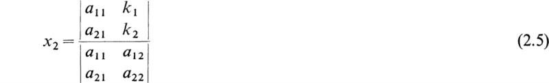
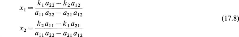
This symbol is called a determinant of the second order. The solution of (2.2) is
Similarly, if we multiply the first equation of (2.1) by — a21 and the second one by a11 and add, we obtain
The expression for the solution of Eqs. (2.1) in terms of the determinants is very convenient and may be generalized to a set of n linear equations in n unknowns. We must first consider the fundamental definitions and rules of operation of determinants and matrices.
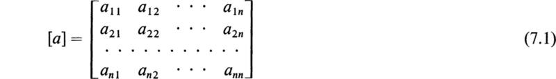
Consider the square array of n2 quantities aij, where the subscripts i and j run from 1 to n, and written in the form
This square array of quantities, bordered by vertical bars, is a symbolical representation of a certain homogeneous polynomial of the nth order in the quantities aij to be defined later and constructed from the rows and columns of |a| in a certain manner. This symbolical representation is called a determinant. The n2 quantities aij are called the elements of the determinant.
In this brief treatment we cannot go into a detailed exposition of the fundamental theorems concerning the homogeneous polynomial that the determinant represents; only the essential theorems that are important to the solution of sets of linear equations will be considered. Before giving explicit rules concerning the construction of the homogeneous polynomial from the symbolic array of rows and columns, it will be necessary to define some terms that are of paramount importance in the theory of determinants.
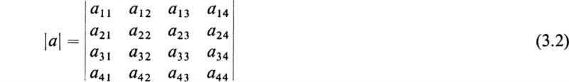
If in the determinant |a| of (3.1) we delete the ith row and the jth column and form a determinant from all the elements remaining, we shall have a new determinant of n — 1 rows and columns. This new determinant is defined to be the minor of the element aij. For example, if |a| is a determinant of the fourth order,
the minor of the element a32 is denoted by M32 and is given by
The cofactor of an element of a determinant aij is the minor of that element with a sign attached to it determined by the numbers i and j which fix the position of aij in the determinant |a|. The sign is chosen by the equation
where Aij is the cofactor of the element aij and Mij is the minor of the element aij.
We come now to a consideration of what may be regarded as the definition of the homogeneous polynomial of the nth order that the symbolical array of elements of the determinant represents. Let us, for simplicity, first consider the second-order determinant
By definition this symbolical array represents the second-order homogeneous polynomial
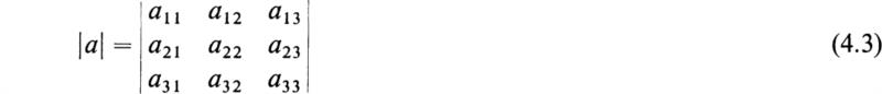
The third-order determinant
represents the unique third-order homogeneous polynomial defined by any one of the six equivalent expressions
where the elements aij in (4.4) must be taken from a single row or a single column of a. The Aij’s are the cofactors of the corresponding elements aij as defined in Sec. 3. As an example of this definition, we see that the third-order determinant may be expanded into the proper third-order homogeneous polynomial that it represents, in the following manner:
This expansion was obtained by applying the fundamental rule (4.4) and expanding in terms of the first row. Since one has the alternative of using any row or any column, it may be seen that (4.3) could be expanded in six different ways by the fundamental rule (4.4). It is easy to show that all six ways lead to the same third-order homogeneous polynomial (4.6).
The definition (4.4) may be generalized to the nth-order determinant (3.1), and this symbol is defined to represent the nth-order homogeneous polynomial given by
where the aij quantities must be taken from a single row or a single column. In this case the cofactors Aij are determinants of the (n – 1)st order, but they may in turn be expanded by the rule (4.7), and so on, until the result is a homogeneous polynomial of the nth order.
It is easy to demonstrate that, in general,
From the basic definition (4.7), the following properties of determinants may be deduced:
a. If all the elements in a row or in a column are zero, the determinant is equal to zero. This may be seen by expanding in terms of that row or column, in which case each term of the expansion contains a factor of zero.
b. If all elements but one in a row or column are zero, the determinant is equal to the product of that element and its cofactor.
c. The value of a determinant is not altered when the rows are changed to columns and the columns to rows. This may be proved by developing the determinant by (4.7).
d. The interchange of any two columns or two rows of a determinant changes the sign of the determinant.
e. If two columns or two rows of a determinant are identical, the determinant is equal to zero.
f. If all the elements in any row or column are multiplied by any factor, the determinant is multiplied by that factor.
g. If each element in any column or any row of a determinant is expressed as the sum of two quantities, the determinant can be expressed as the sum of two determinants of the same order.
h. Is it possible, without changing the value of a determinant, to multiply the elements of any row (or any column) by the same constant and add the products to any other row (or column). For example, consider the third-order determinant
With the aid of property g we have
Since the second determinant is zero because the first and third columns are identical, we have
The evaluation of determinants whose elements are numbers is a task of frequent occurrence in applied mathematics. This evaluation may be carried out by a direct application of the fundamental Laplacian expansion (4.7). This process, however, is most laborious for high-order determinants, and the expansion may be more easily effected by the application of the fundamental properties outlined in Sec. 5 and by the use of two theorems that will be mentioned in this section.
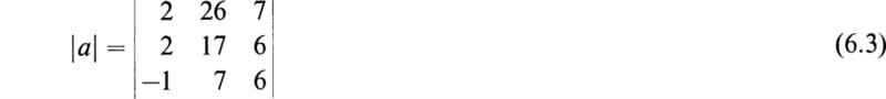
As an example, let it be required to evaluate the numerical determinant
This determinant may be transformed by the use of property b of Sec. 5. The procedure is to make all elements but one in some row or column equal to zero. The presence of the factor —1 in the second column suggests that we add four times the first row to the second, then add two times the first row to the third row, and finally add the first row to the fourth row. By Sec. 5h these operations do not change the value of the determinant. Hence we have
If we now subtract the elements of the last column from the first column, we have
We now add two times the third row to the first row and two times the third row to the second row and obtain
Now we may subtract the second row from the first row and obtain
This procedure is much shorter than a direct application of the Laplacian expansion rule.
We now turn to a consideration of a theorem of great power for evaluating numerical determinants. The method of evaluation, based on the theorem to be considered, was found most successful at the Mathematical Laboratory of the University of Edinburgh and was due originally to F. Chiò.
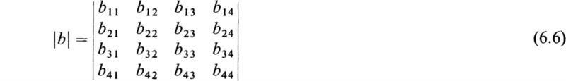
To deduce the theorem in question, consider the fourth-order determinant
We now notice whether any element is equal to unity. If not, we prepare the determinant in such a manner that one of the elements is unity. This may be done by dividing some row or column by a suitable number, say m, that will make one of the elements equal to unity and then placing the number m as a factor outside the determinant. The same result may also be effected in many cases with the aid of Sec. 5h. For simplicity we shall suppose that this has been done and that, in this case, the element b23 is equal to unity.
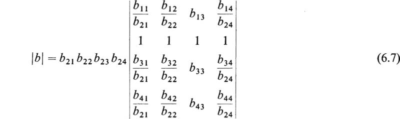
Now let us divide the various columns of the determinant b by b21 b22, b23, and b24, respectively; then in view of the fact that the element b23 has been made unity, we have
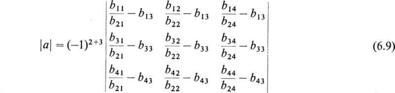
Now, if we subtract the elements of the third column from those of the other columns, we obtain

Expanding in terms of the second row, we obtain
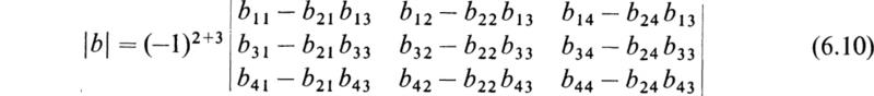
Substituting this value of |a| into (6.8) and multiplying the various columns by the factors outside, we finally obtain
The theorem may be formulated by means of the following rule. The element that has been made unity at the start of the process is called the pivotal element. In this case it is the element b23. The rule says:
The row and column intersecting in the pivotal element of the original determinant, say the rth row and the sth column, are deleted; then every element u is diminished by the product of the elements which stand where the eliminated row and column are met by perpendiculars from u, and the whole determinant is multiplied by (–1)r+s.
By the application of this theorem we reduce the order of the determinant by one unit. Repeated application of this theorem reduces the determinant to one of the second order, and then its value is immediately written down.
Before turning to a consideration of linear algebraic equations and to the application of the theory of determinants to their solution, a brief discussion of matrix algebra and the fundamental operations involving matrices is necessary. In this chapter the fundamental definitions and the most important properties of matrices will be outlined.
By a square matrix a of order n is meant a system of elements that may be real or complex numbers arranged in a square formation of n rows and columns. That is, the symbol [a] stands for the array
where aij denotes the element standing in the ith row and jth column. The determinant having the same elements as the matrix [a] is denoted by |a| and is called the determinant of the matrix.
Besides square arrays like (7.1) we shall have occasion to use rectangular arrays or matrices of m rows and n columns. Such arrays will be called matrices of order (m × n). Where there is only one row so that m = 1, the matrix will be termed a vector of the first kind, or a prime. As an example, we have
On the other hand, a matrix of a single column of n elements will be termed a vector of the second kind, or a point. To save space, it will be printed horizontally and not vertically and will be denoted by parentheses thus:
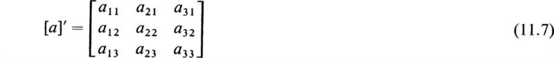
The accented matrix [a]′ = [aji] obtained by a complete interchange of rows and columns in [a] is called the transposed matrix of [a]. The ith row of [a] is identical with the ith column of [a]′. For vectors we have
For rectangular matrices the transpose is
a. Square matrix: If the numbers of rows and of columns of a matrix are equal to n, then such a matrix is said to be a square matrix of order n, or simply a matrix of order n.
b. Diagonal matrix: If all the elements other than those in the principal diagonal are zero, then the matrix is called a diagonal matrix.
c. The unit matrix: The unit matrix of order n is defined to be the diagonal matrix of order n which has l’s for all its diagonal elements. It is denoted by Un or simply by U when its order is apparent.
d. Symmetrical matrices: If aij = aji for all i and j, the matrix [a] is said to be symmetrical and it is identical to its transposed matrix. That is, if [a] is symmetrical, then [a]′ = [a], and conversely.
e. Skew-symmetric matrix: If aij = —aji for all unequal i and j, but the elements aii are not all zero, then the matrix is called a skew matrix.
If aij = —aji for all i and j so that all aii = 0, the matrix is called a skew-symmetric matrix. It may be noted that both symmetrical and skew matrices are necessarily square.
f. Null matrices: If a matrix has all its elements equal to zero, it is called a null matrix and is represented by [0].
It is apparent from what has been said concerning matrices that a matrix is entirely different from a determinant. A determinant is a symbolic representation of a certain homogeneous polynomial formed from the elements of the determinant as described in Sec. 4. A matrix, on the other hand, is merely a square or rectangular array of quantities. By defining certain rules of operation that prescribe the manner in which these arrays are to be manipulated, a certain algebra may be developed that has a formal similarity to ordinary algebra but involves certain operations that are performed on the elements of the matrices. It is to a consideration of these fundamental definitions and rules of operation that we now turn.
The concept of equality is fundamental in algebra and is likewise of fundamental importance in matrix algebra. In matrix algebra two matrices [a] and [b] of the same order are defined to be equal if and only if their corresponding elements are identical; that is, we have
provided that
If [a] and [b] are matrices of the same order, then the sum of [a] and [b] is defined to be a matrix [c], the typical element of which is cij = aij + bij. In other words, by definition
In a similar manner we have
provided that
By definition, multiplication of a matrix [a] by an ordinary number or scalar k results in a new matrix b defined by
where
That is, by definition, the multiplication of a matrix by a scalar quantity yields a new matrix whose elements are obtained by multiplying the elements of the original matrix by the scalar multiplier.
The definition of the operation of multiplication of matrices by matrices differs in important respects from ordinary scalar multiplication. The rule of multiplication is such that two matrices can be multiplied only when the number of columns of the first is equal to the number of rows of the second. Matrices that satisfy this condition are termed conformable matrices.
Definition The product of a matrix [a] by a matrix [b] is defined by the equation
where
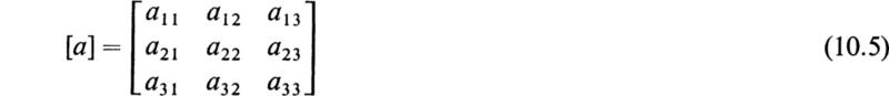
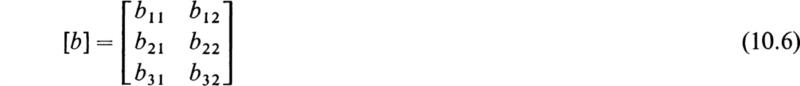
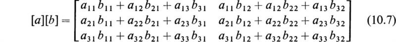
and the orders of the matrices [a], [b], and [c] are (m × p), (p × n), and (m × n), respectively. As an example of this definition, let us consider the multiplication of the matrix
By applying the definition we obtain
If the matrices are square and each of order n, then the corresponding relation |a| |b| = |c| is true for the determinants of the matrices [a], [b], and [c]. The proof of this frequently useful result will be omitted.
Since matrices are regarded as equal only when they are element for element identical, it follows that, since a row-by-column rule will, in general, give different elements than a column-by-row rule, the product [b][a], when it exists, is usually different from [a][b]. Therefore it is necessary to distinguish between premultiplication, as when [b] is premultiplied by [a] to yield the product [a][b], and postmultiplication, as when [b] is postmultiplied by [a] to yield the product [b][a]. If we have the equality
the matrices a and b are said to commute or to be permutable. The unit matrix U, it may be noted, commutes with any square matrix of the same order. That is, we have for all such [a]
Except for the noncommutative law of multiplication (and therefore of division, which is defined as the inverse operation), all the ordinary laws of algebra apply to matrices. Of particular importance is the associative law of continued products,
which allows one to dispense with parentheses and to write [a][b][c] without ambiguity, since the double summation
![]()
can be carried out in either of the orders indicated.
It must be noted, however, that the product of a chain of matrices will have meaning only if the adjacent matrices of the chain are conformable.
If a square matrix is multiplied by itself n times, the resultant matrix is defined as [a]n. That is,
If the determinant |a| of a square matrix [a] does not vanish, [a] is said to be nonsingular and possesses a reciprocal, or inverse, matrix [R] such that
where U is the unit matrix of the same order as [a].
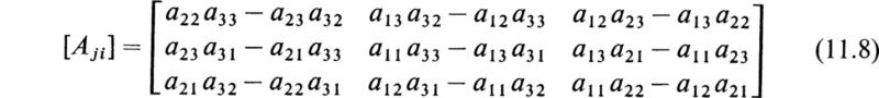
Let Aij denote the cofactor of the element aij in the determinant |a| of the matrix [a]. Then the matrix [Aji] is called the adjoint of the matrix [a]. This matrix exists whether [a] is singular or not. Now by (4.8) we have
It is thus seen that the product of [a] and its adjoint is a special type of diagonal matrix called a scalar matrix. Each diagonal element i = j is equal to the determinant |a|, and the other elements are zero.
If |a| ≠ 0, we may divide through by the scalar |a| and hence obtain at once the required form of [R], the inverse of [a]. From (11.2) we thus have
Therefore, comparing this with (11.1) we see that
The notation [a]–1 is introduced to denote the inverse of [a]. By actual multiplication it may be proved that
so that the name reciprocal and the notation [a]–1 are justified.
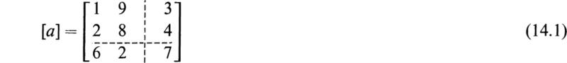
If a square matrix is nonsingular, it possesses a reciprocal, and multiplication by the reciprocal is in many ways analogous to division in ordinary algebra. As an illustration, let it be required to obtain the inverse of the matrix
Let |a| denote the determinant of [a]. The next step in the process is to form the transpose of a.
We now replace the elements of [a]′ by their corresponding cofactors and obtain
This inverse [a]–1 is therefore
As has been mentioned, multiplication by an inverse matrix plays the same role in matrix algebra that division plays in ordinary algebra. That is, if we have
where [a] is a nonsingular matrix, then, on premultiplying by [a]-1, the inverse of [a], we obtain
or
If [a] is a nonsingular matrix, then negative powers of [a] are defined by raising the inverse matrix of [a], [a]–1, to positive powers. That is,
One of the fundamental consequences of the noncommutative law of matrix multiplication is the reversal law exemplified in transposing and reciprocating a continued product of matrices.
Let [a] be a (p × n) matrix, that is, one having; p rows and n columns, and let [b] be an (m × p) matrix. Then the product [c] = [b][a] is an (m × n) matrix of which the typical element is
When transposed, [a]′ and [b]′ become (n ×p) and (p × m) matrices; they are now conformable when multiplied in the order [a]′[b]′. This product is an (n × m) matrix, which may be readily seen to be the transpose of [c] since its typical element is
It thus follows that when a matrix product is transposed the order of the matrices forming the product must be reversed. That is,
and similarly
Let us suppose that in the equation [c] = [b][a] the matrices are square and nonsingular. If we premultiply both sides of the equation by [a]–1[b]–1 and postmultiply by [c]–1, then we obtain [a]–1[b]–1 = [c]–1. We thus get the rule that
Similarly
Suppose that [a] is a square matrix of order n and [b] is a diagonal matrix, that is, a matrix that has all its elements zero with the exception of the elements in the main diagonal, and is of the same order as [a]. Then, if [c] = [b][a], we have
since bir = 0 unless r = i.
It is thus seen that premultiplication by a diagonal matrix has the effect of multiplying every element in any row of a matrix by a constant. It can be similarly shown that postmultiplication by a diagonal matrix results in the multiplication of every element in any column of a matrix by a constant. The unit matrix plays the same role in matrix algebra that the number 1 does in ordinary scalar algebra.
It is sometimes convenient to extend the use of the fundamental laws of combinations of matrices to the case where a matrix is regarded as constructed from elements that are submatrices or minor matrices of elements. As an example, consider
This can be written in the form
where

In this case the diagonal submatrices [P] and [S] are square, and the partitioning is diagonally symmetrical. Let [b] be a square matrix of the third order that is similarly partitioned.
Then, by addition and multiplication, we have
as may be easily verified.
In each case the resulting matrix is of the same order that is partitioned in the same way as the original matrix factors. As has been stated in Sec. 10, a rectangular matrix [b] may be premultiplied by another rectangular matrix [a] provided the two matrices are conformable, that is, the number of rows of [b] is equal to the number of columns of [a]. Now, if [a] and [b] are both partitioned into submatrices such that the grouping of columns in [a] agrees with the grouping of rows in [b], it can be shown that the product [a][b] may be obtained by treating the submatrices as elements and proceeding according to the multiplication rule.
a. Conjugate matrices: To the operations [a]′ and [a]–1, defined by transposition and inversion, may be added another one. This operation is denoted by [ā] and implies that if the elements of [a] are complex numbers, the corresponding elements of [ā] are their respective complex conjugates. The matrix [ā] is called the conjugate of [a].
b. The associate of [a]: The transposed conjugate of [a], [ā]′, is called the associate of [a].
c. Symmetric matrix: If [a] = [a]′, the matrix [a] is symmetric.
d. Involutory matrix: If [a] = [a]–1, the matrix [a] is involutory.
e. Real matrix: If [a] = [ā], [a] is a real matrix.
f. Orthogonal matrix: If [a] = ([a]′)–1, [a] is an orthogonal matrix.
g. Hermitian matrix: If [a] = [ā], [a] is a Hermitian matrix.
h. Unitary matrix: If [a] = ([ā]′)–1, [a] is unitary.
i. Skew-symmetric matrix: If [a] = —[a]′, [a] is skew symmetric.
j. Pure imaginary: If [a] = —[ā], [a] is pure imaginary.
k. Skew Hermitian: If [a] = —[ā]′, [a] is skew Hermitian.
Prior to discussing the solution of a system of linear algebraic equations, the rank of a matrix must be defined. The rank† of a matrix is equal to the order of the largest nonvanishing determinant contained within the matrix. Thus the ranks of
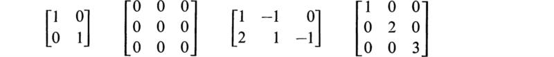
and
are 2, 0, 2, 3, and 2, respectively.
The concept of rank is not restricted to square matrices, as can be seen in the third example above. For the case of square matrices, it is easily seen that if the rank equals the order of the matrix, then it necessarily has an inverse.
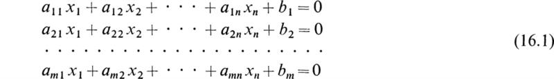
Now to move to the subject of this section we shall consider a non-homogeneous system of m linear algebraic equations and n unknowns:
Using matrix notation, the above system reduces to
where [A] = mxn coefficient matrix

Another useful matrix is the mx(n + l)-augmented matrix defined by
This particular matrix is formed by attaching the vector of known constants as an additional column on the coefficient matrix.
The system of equations defined by (16.2) is said to be consistent if a solution vector {x} exists which satisfies the system. If no solution exists, then the system is said to be inconsistent.† We are now at a point where we may present the conditions, without proof,‡ under which the system (16.2) will be consistent. These conditions may be grouped into the following three categories:
1. Rank of [A] = rank [A,b] = ![]() This situation yields a solution for any r unknowns in terms of the n — r remaining ones.
This situation yields a solution for any r unknowns in terms of the n — r remaining ones.
2. Rank of [A] = rank of [A,b] = r = n: This situation yields a unique solution for the n unknowns.
3. Rank of [A] = rank of [A,b] = r < n: A solution always exists in this case.
It should be noted that in each of the above conditions the ranks of the coefficient and augmented matrices were equal. This in fact is the basic and only requirement for the existence of a solution to (16.2). Reiterating this statement, it can be proven§ that a system of linear algebraic equations is consistent if and only if the rank of the coefficient matrix equals the rank of the augmented matrix.
When m = n in (16.2), we have the special case of a system of n linear algebraic equations and n unknowns. As in any case a solution will only exist when the ranks of the coefficient and augmented matrices are equal. For convenience we shall assume that the ranks of both of these matrices equal n. This allows us to premultiply by the inverse of the coefficient matrix to obtain the solution.
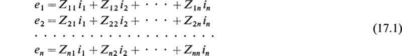
Suppose we have the set of n linear algebraic equations in n unknowns,
The quantities ej, Zij, and ij may be real or complex numbers. If the relation (17.1) exists between the variables ej and ij, then the set of variables ej is said to be derived from the set ij by a linear transformation. The whole set of Eqs. (17.1) may be represented by the single matrix equation
where {e} and {i} are column matrices whose elements are the variables ej and ij. The square matrix [Z] is called the matrix of the transformation. When [Z] is nonsingular, Eq. (17.2) may be premultiplied by [Z]–1 and we obtain
We thus have a very convenient explicit solution for the unknowns (i1, i2, . . . ,in). The elements of the matrix [Z]–1 may be calculated by Eq. (11.4). As a simple example, let us solve the system of Eqs. (2.1) by using matrix notation. If we introduce the matrices
then Eqs. (2.1) may be written in the form
and if [a] is nonsingular, the solution is
But by (11.4) we have
Hence, carrying out the matrix multiplication expressed in (17.6), we obtain
Although the solution of a set of linear equations is very elegantly and concisely expressed in terms of the inverse matrix of the coefficients, it frequently happens in practice that it is necessary to solve for only one or two of the unknowns.
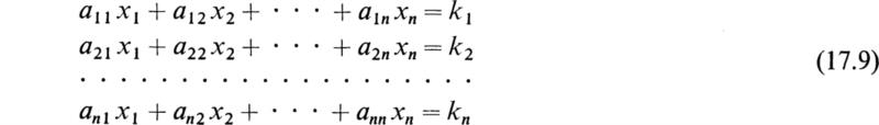
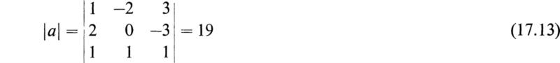
In this case it is frequently more convenient to use Cramer’s rule to obtain the solution. The proof of Cramer’s rule follows from the properties of the determinant expressed by Eq. (4.8) and will not be given. Let us consider the set of n equations in the unknowns (x1, x2, . . . ,xn),
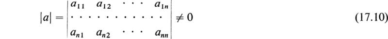
Then if the determinant of the system
the system of Eqs. (17.9) has a unique solution given by
where Dr is the determinant formed by replacing the elements
![]()
of the rth column of |a| by (k1, k2, . . . , kn), respectively.
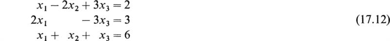
For example, let us solve the system
Hence
At the risk of repeating what has already been stated in Sec. 16, we shall review some special cases that may arise when working with a system of n equations and n unknowns.
1. If the determinant |a| ≠ 0, there exists a unique solution that is given by Cramer’s rule, that is, (17.11).
2. If a is of rank r < n and any of the determinants D1, D2, . . . , Dn of (17.11) are of rank greater than r, there is no solution.
3. If |a| is of rank r < n and the rank of none of D1 D2, . . . , Dn exceeds r, then there exist infinitely many sets of solutions.
If in Eq. (16.2) the vector {b} is a null vector, that is {b} = {0}, then (16.2) reduces to the following system of homogeneous linear equations:
Regardless of the order of [A], this system is consistent; hence a solution always exists. By inspection it is easy to see that the solution vector {x} = {0} satisfies (18.1) identically. This particular solution is called the trivial solution. In most cases this solution is of little interest to the analyst, and other solutions called nontrivial solutions are sought.
In the most general case the matrix [A] is of order m × n; however, it usually is n × n. In either case it may be stated that if the rank of [A] is less than n, then a nontrivial solution to (18.1) exists. In the case when the rank of the coefficient matrix is n, the only solution that exists is the trivial one.
A few examples of solutions to homogeneous systems are given below.
Example 1
The rank of [A] in this case is 2 and n = 2, hence only the trivial solution exists.
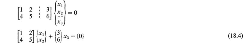
Example 2
In this case the rank of the coefficient matrix is 2, but n = 3; thus a nontrivial solution exists. To obtain the solution we proceed as follows. Since the rank of [A] is 2 and there are three unknowns, then any two unknowns may be solved for in terms of the third. This may be accomplished in a variety of ways, one of which is the following.
By partitioning, write (18.3) as
If we premultiply this equation through by
![]()
and solve for the vector
![]()
we find the following solution:

or
![]()
The complete solution may be written in vector form as
where c represents an arbitrary constant.
If μ is a scalar parameter and [M] is a square matrix of order n, the matrix
U = the nth-order unit matrix, is called the characteristic matrix of the matrix [M]. The determinant of the characteristic matrix, det [K], is called the characteristic function of [M]. That is,
is the characteristic function of the matrix [M].
The equation
is the characteristic equation of the matrix [M]. In general, if [M] is a square matrix of the nth order, its characteristic equation is an equation of the nth degree in μ.
The n roots of this equation are called the characteristic roots, or eigenvalues, of the matrix [M].
In matrix algebra, when a matrix contains only one column, it is called a column vector. If {x} is a column vector of the nth order and [M] is an nth-order square matrix, the product
expresses the fact that the vector {y} is derived from the vector {x} by a linear transformation. The square matrix [M] is called the transformation matrix. If it is required that
then (20.1) reduces to
and the only effect of the transformation matrix [M] on the vector {x} is to multiply it by the scalar factor μ. Equation (20.3) may be written in the form
This equation represents a set of homogeneous linear equations in the unknowns x1, x2, . . . , xn. Except in the trivial case where all the elements of {x} are zero, the determinant of [K] must vanish. Conversely, if |K| =0, there exist nontrivial solutions. In order for this to be the case, the scalar μ can take only the values μ1, μ2, . . . , μn which are the roots of the characteristic equation (19.3). The possible values of μ which satisfy (20.3) are thus the eigenvalues of [M], The nontrivial solutions of (20.4) associated with these eigenvalues are called eigenvectors of [M].
To each eigenvalue μi there corresponds an equation of the form (20.3) which can be written as follows :
where {x}i is any eigenvector associated with μi.
If (20.5) is premultiplied by [M], it becomes
By repeated multiplications by [M] it can be shown that
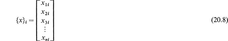
Let the ith eigenvector be denoted by
and let the square matrix [x] be the matrix formed by grouping the column eigenvectors into a square matrix so that
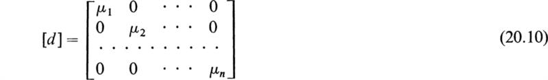
If (d) denotes the square diagonal matrix
it can be seen that the set of n equations (20.5) may be written in the form
If the n eigenvalues of [M] are distinct, it can be shown that the matrix [x] is nonsingular and possesses an inverse [x]–1.† Hence (20.11) may be written in the form
or
It is thus seen that a matrix [x] which diagonalizes [M] may be found by grouping the eigenvectors of [M] into a square matrix. This may be done when the eigenvalues of [M] are all different. When two or more of the eigenvalues of [M] are equal to each other, reduction to the diagonal form is not always possible.
The sum of all the diagonal elements of a square matrix is called the trace of the matrix and is denoted by the following expression:
There exist some interesting relations between the trace of a matrix and the characteristic equation of the matrix.‡ The characteristic equation of [M] has the form
It can be shown that
If μ1, μ2, . . . , μn are the eigenvalues of [M], then as a result of (21.3) we have
It can be shown that the product of the eigenvalues is given by the equation
Maxime Bôcher has shown that there is an intimate connection between the traces of powers of a matrix and the coefficients of its characteristic equation (21.2) These results are of importance in obtaining the characteristic equations of matrices and in the computation of the inverses of matrices. The results of Bôcher are deduced in his book on higher algebra and are given here without proof.
The characteristic equation of a square matrix [M] of the nth order is, in general, an equation of the nth degree as given by (21.2). Bôcher’s results relate the coefficients ci of the characteristic equation of [M] to the traces of powers of [M]. Let
Then the coefficients c1 c2, . . . , cn of the characteristic equations are
These equations enable one to obtain the characteristic equation of a matrix in a more efficient manner than by the direct expansion of det [μU— M]. If the determinant of [M] itself is desired, it can be calculated by the use of the following equation:
where cn is as given above.
One of the most important theorems of the theory of matrices is the Cayley-Hamilton theorem. By the use of this theorem many properties of matrices may be deduced, and functions of matrices can be simplified. The Cayley-Hamilton theorem is frequently stated in the following terse manner: Every square matrix satisfies its own characteristic equation in a matrix sense. This statement means that if the characteristic equation of the nth-order matrix [M] is given by
the Cayley-Hamilton theorem states that
where U is the nth-order unit matrix.
A heuristic proof of this theorem may be given by the use of the following result of Sec. 20:
where μi is the ith eigenvalue of [M] and {x}i is the corresponding eigenvector. The characteristic function of [M] is given by
If in (22.4) the scalar μ is replaced by the square matrix [M] and the coefficient of cn is multiplied by the nth-order unit matrix U, the result may be written in the following form:
If (22.5) is postmultiplied by the eigenvector {x}i the result is
As a consequence of (22.3), this may be written in the following form:
However, since μi is one of the eigenvalues of [M], we have
Hence (22.7) reduces to
The set of equations (22.9) may be written as the single equation
where [x] is the square matrix (20.9) and [0] is an nth-order square matrix of zeros. If [M] has n distinct eigenvalues, the matrix [x] is nonsingular and has an inverse. If (22.10) is postmultiplied by [x]–1, the result is
This important result is the Cayley-Hamilton theorem. It may be shown that the Cayley-Hamilton theorem holds for singular matrices and for matrices that have repeated eigenvalues.†
If the matrix [M] is nonsingular, its inverse may be computed by the use of the Cayley-Hamilton theorem in the following manner: Expand (22.11) in the form
If this equation is premultiplied by [M]–1, the result is
Hence, if this equation is solved for [M]–1, the result is
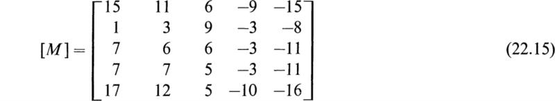
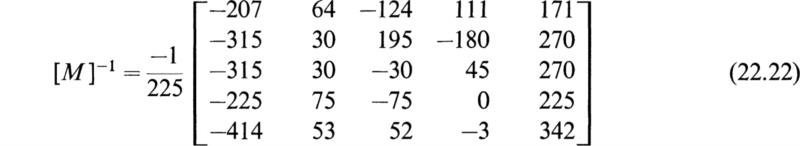
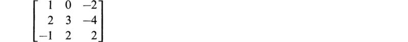
This result expresses the inverse of [M] in terms of the n — 1 powers of [M] and has been suggested as a practical method for the computation of the inverses of large matrices.† Hotelling gives the following application of (22.14) to the computation of the inverse of a numerical matrix: Let the matrix to be inverted be
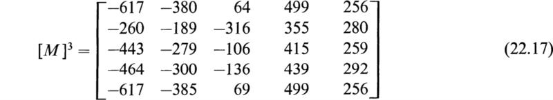
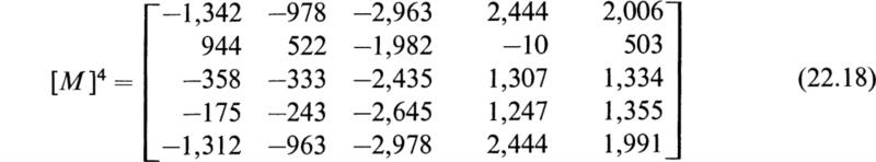
Then
From the diagonals of the above matrices, the following traces may be calculated:
By means of (21.7) the following coefficients of the characteristic equation of [M] can be computed:
The characteristic equation of [M] is therefore
The inverse of [M] is now computed by the use of (22.14) and is given by
If the determinant of [M] is desired, it may be obtained from the equation
This method for the computation of the inverse of a matrix is straightforward and easily checked and is ideally adapted to matrix multiplication by means of punched cards. As a by-product of the computation the characteristic equation and the determinant of the matrix are obtained.
With the development of many powerful modern instruments of calculation such as punched-card machines, electronic digital-computing machines, analogue computers, etc., the field of application of mathematical analysis has vastly increased. Many diversified problems in various fields may be reduced to one mathematical operation: that of the solution of systems of linear algebraic equations. A few of the problems that may be reduced to this mathematical common denominator are the following:
1. The distribution of electrical currents in multimesh electrical circuits.
2. The distribution of the rate of flow of water in complex hydraulic systems.
3. The approximate solution of potential problems.
4. The solution of the normal equations in the application of the method of least squares to various physical investigations.
5. The applications of statistical studies to psychology, sociology, and economics.
6. The determination of the amplitudes of motion in the forced vibrations of mechanical systems.
7. The approximate solution of certain problems of electromagnetic radiation.
The above list is far from complete, but it gives an indication of the diversified classes of problems that may be reduced to the solution of a system of linear equations.
It may be thought that the problem of solving systems of linear equations is an old one and that it can be effected by means of well-known techniques such as Cramer’s rule (Sec. 16). However, in studying problems of the type enumerated above, it is frequently necessary to solve 150 or 200 simultaneous equations. This task presents practically insurmountable difficulties if undertaken by well-known elementary methods. In the past few years many powerful and apparently unrelated methods have been devised to perform this task. A very complete survey of these methods, with a bibliography containing 131 references, will be found in the paper by Forsythe.†
The magnitude of the task of solving a large system of linear equations by conventional elementary methods and the spectacular reduction of effort that may be effected by the use of modern techniques are vividly presented by Forsythe. He points out that the conventional Cramer’s-rule procedure for solving n simultaneous equations requires the evaluation of n + 1 determinants. If these determinants are evaluated by the Laplace expansion (Sec. 4), this requires n! multiplications per determinant. It is thus apparent that the conventional determinantal method of solution requires (n + 1)! multiplications. Therefore, if it is required to solve 26 equations, it would, in general, require (n + 1)! = 27! ≈ 1028 multiplications. A typical high-speed digital machine such as the IBM/360 model 75 automatic computer can perform 133,000 multiplications per second. Hence, it would take this machine approximately 1014 years to effect the solution of this problem by the use of the conventional Cramer’s-rule technique. By more efficient techniques the computational procedure may be arranged so that only about n3/3 multiplications are required to solve the system of n equations. If this efficient method is used, 6,000 multiplications would be required, and the IBM machine can solve the problem in about 0.05 sec.
The detailed theory of the various methods that have been developed in recent years will be found in the above survey article by Forsythe and should be consulted by those interested in the solution of large numbers of simultaneous linear equations. A simple method that has been found valuable and that makes use of partitioned matrices will now be described.
Let the matrix whose inverse is desired be the matrix [M], of order n. Then, by the methods of Sec. 14, the matrix [M] can be partitioned into four submatrices in the following manner:
The orders of the various matrices are indicated by the letters in parentheses. The first letter denotes the number of rows and the second letter the number of columns. Since the original matrix is of order n, we have the relation
Now let the reciprocal of [M] be the matrix [B], and let it be correspondingly partitioned so that we have
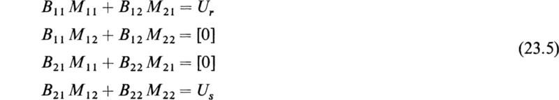
Since [B] is the inverse of [M], we have
where Un is the unit matrix of order n. If the multiplication indicated by (23.4) is carried out, we have
These equations may, in general, be solved to give the submatrices of the required matrix [B] explicitly. The results may be expressed as follows: Let
We then have explicitly
These equations determine [B] = [M]–1 provided that the reciprocals ![]() and θ–1 exist. If
and θ–1 exist. If ![]() known, then the matrices X, Y, and θ can be calculated by matrix multiplication and [B] can be determined by the use of (23.7). The choice of the manner in which the original matrix [M] is partitioned depends on the particular matrix to be inverted. From the above description of the method it is obvious that it yields to various modifications. The method of Sec. 22 may advantageously be applied to find
known, then the matrices X, Y, and θ can be calculated by matrix multiplication and [B] can be determined by the use of (23.7). The choice of the manner in which the original matrix [M] is partitioned depends on the particular matrix to be inverted. From the above description of the method it is obvious that it yields to various modifications. The method of Sec. 22 may advantageously be applied to find ![]() and θ–1. By this procedure the inversion of a large matrix may be reduced to the inversion of several smaller matrices.
and θ–1. By this procedure the inversion of a large matrix may be reduced to the inversion of several smaller matrices.
Another very effective method for the inversion of matrices is Choleski’s method. In its simplest form it applies to the inversion of symmetric matrices and is simple in theory and straightforward in practice. This method is sometimes called the square-root method, and an excellent exposition of this method is given in the paper by Fox, Huskey, and Wilkinson.† Choleski’s method consists simply in expressing the symmetric matrix [M] whose inverse is desired in the form
where [L] is a lower triangular matrix and [L], its transpose, an upper triangular matrix. Then the desired inverse is given by
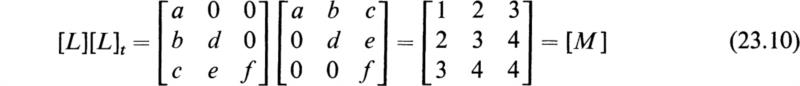
and the problem is solved. To fix the fundamental ideas involved, consider the case of a third-order symmetric matrix [M]. We then have to find the third-order matrices [L] and [L]t by means of the equation
By matrix multiplication of [L][L]t the following result is obtained:
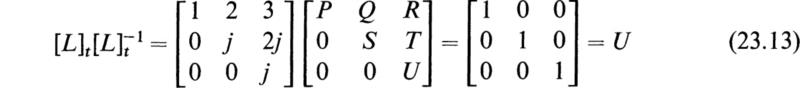
By equating the elements of [L]|L]t to those of [M] and solving the resulting equations one finds a=1, b = 2, c = 3, d=j, e = 2j, f=j. In order to determine [M]–1 by (23.9), it is necessary to invert [L]t. This is easily done because ![]() is also an upper triangular matrix of the form
is also an upper triangular matrix of the form
The elements of ![]() may be determined by the equation
may be determined by the equation
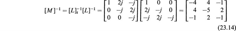
From (23.13) we find that P=l, Q = 2j, R = –j, S = –j, T=2j, U = –j. The required inverse of [M] is given by
The work involved in the Choleski method appears formidable in the above example but in practice can be greatly reduced. The method can be extended to the computations of inverses of unsymmetric matrices.
A very important and useful theorem of matrix algebra is known as Sylvester’s theorem. This theorem states that, if the n eigenvalues μ1 μ2, . . . , μn of the square matrix [M] are all distinct and P([M]) is a polynomial in [M] of the following form:
where U is the nth-order unit matrix and the ck’s are constants, then the polynomial P([M]) may be expressed in the following form:
where
In (24.3) ∆(μ) is the characteristic function of [M] as defined by (19.2); [A(μ)] is the adjoint matrix of the characteristic matrix of [M] defined by
and
A proof of Sylvester’s theorem as well as the confluent form of the theorem in the case that the matrix [M] does not have distinct eigenvalues will be found in the book by Frazer, Duncan, and Collar.†
Sylvester’s theorem is very useful for simplifying the calculations of powers and functions of matrices. For example, let it be required to find the value of [M]256, where
To do this, consider the special polynomial
and apply the results of Sylvester’s theorem. In this special case we have
and
The eigenvalues of [M] are μ1 = 1 and μ2 = 3. [A(μ)] is now given by
and
Hence we have
Therefore, by Sylvester’s theorem, we have
As the last step above suggests, Sylvester’s theorem is very useful in obtaining the approximate value of a matrix raised to a high power. Thus, if μm is the largest eigenvalue of the square matrix [M], then, if k is very large, the term P(μm)Z0(μm) will dominate the right-hand member of (24.2) and we have the following approximate value of [M]k:
This expression is useful in certain applications of matrix algebra to physical problems.
A series of the type
where [M] is a square matrix of order n, the coefficients ct are ordinary numbers, and [M]0 = U, the nth-order unit matrix, is called a power series of matrices. The general question of the convergence of such series will not be discussed here; however, if [M] is a square matrix of order n, it is clear that by the use of the Cayley-Hamilton theorem (Sec. 22) it is possible to reduce any matrix polynomial of [M] to a polynomial of maximum degree n — 1 regardless of the degree of the original polynomial. Hence, if the series (25.1) converges,† it may be expressed in the following form:
where
as a consequence of Sylvester’s theorem (Sec. 24). For example, it can be shown that the series
converges for any square matrix [M]. In particular, suppose that the matrix [M] is the following second-order matrix:
The characteristic equation of this matrix is
so that the eigenvalues of [M] are μ1 = 1, μ2 = 2. The matrix [A(μ)] is now
Since ∆′(1) = –1 and ∆′(2) = +1, we have as a consequence of (25.2)
Other functions of matrices such as trigonometric, hyperbolic, and logarithmic functions are defined by the same power series that define these functions for scalar values of their arguments and by replacing these scalar arguments by square matrices. For example, we have
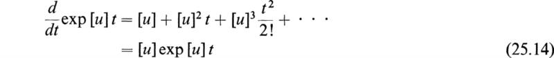
Although every scalar power series has its matrix analogue, the matrix power series have, in general, more complex properties. The properties of the matrix functions may be deduced from their series expansions. For example, if t is a scalar variable and [u] is a square matrix of constants, we have
The series obtained by the term-by-term differentiation of (25.13) is
In the same way, it may be shown that, if
then
In Sec. 25 we saw how Sylvester’s theorem could be used to evaluate functions of matrices. This process, though useful, is sometimes tedious in its application. In this section an alternate method is presented which is generally more convenient to use.
In Sec. 22 it was seen how any matrix polynomial of order n could be reduced to a polynomial of order n — 1 by applying the Cayley-Hamilton theorem. Since any function of a matrix of order n may be represented by an infinite series, the Cayley-Hamilton theorem allows us to assert that any matrix function of order n may be expressed in terms of a polynomial of order n — 1; that is,
where [A] is of order n.
The coefficients ai in (26.1) are unknown, and the problem is to determine them. Resorting again to the Cayley-Hamilton theorem, we assert that for each eigenvalue of [A], μi, we must have
Equation (26.2) yields n equations for the n unknowns ai. Employing matrix notation, (26.2) may be expressed as
or more simply
where the element Fi denotes F(μi) and [V] is the Vandermonde matrix of eigenvalues.
As long as all the eigenvalues are distinct, the matrix [V] has an inverse and hence we may solve for the unknowns ai:
As a first example let us evaluate

which was done in Sec. 25 by application of Sylvester’s theorem. According to (26.1), we may write
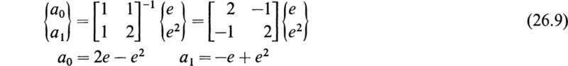
The eigenvalues of [M] are 1 and 2; thus by (26.2) we have
Inverting and solving for a0 and a1 yields
Substituting into (26.6) gives
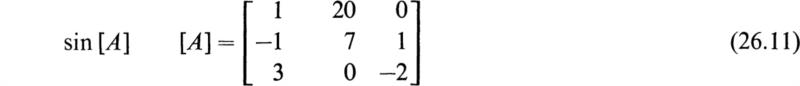
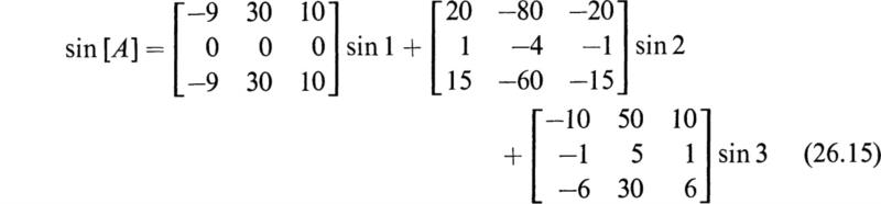
As a second example consider the problem of evaluating
The reader may verify that the eigenvalues of A are 1, 2, and 3, respectively. By (26.1) we may write
Substituting into (26.2) yields
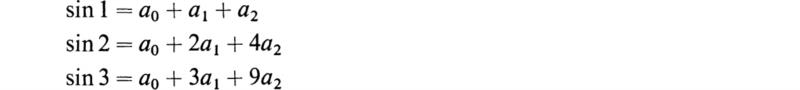
or in the form of (26.3)
Solving for the vector {a} gives
from which a0, a1 and a2 may be found. Substituting these values into (26.12) yields the final result:
Up to this point we have considered the elements of the matrices as constants, which is the most common situation. However, in the theory of matrix differential equations, cases frequently arise wherein the elements of the matrices are functions of the independent variable, e.g., time.
If, for example, we consider a matrix whose elements are functions of time, then we can define the derivative and integral of such a matrix as follows:
In other words, the derivative or integral of a matrix is the matrix of the derivatives or integrals of the individual elements. The requirement for the existence of the derivative or integral of a matrix is simply that the derivative or integral of every element must exist.
A very important field of application of the theory of matrices is the solution of systems of linear differential equations. Matrix notation and operations with matrices lead to concise formulations of otherwise cumbersome procedures. This conciseness is very important in many practical problems that involve several dependent variables. Such problems arise in dynamics, the theory of vibrations of structures and machinery, the oscillations of electrical circuits, electric filters, and many other branches of physics and engineering.
In order to apply matrix notation to a set of differential equations, it is advisable to express the equations in forms that involve only the first-order differential coefficients. Any set of differential equations can be easily changed into another set that involves only first-order differential coefficients by writing the highest-order coefficient as the differential coefficient of a new dependent variable. All the other differential coefficients are regarded as separate dependent variables, and, for each new variable introduced, another equation must be added to the set. As a very simple example, consider the following equation:
In order to express this as a set of first-order equations, let x = x1 and
With this notation (28.1) becomes
Therefore the original second-order differential equation (28.1) may be written in the following matrix form:
This is a special case of the first-order matrix differential equation d.
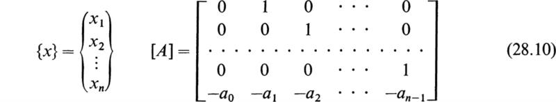
where {x} is in general a column vector of the n elements x1 x2, . . . , xn and [A] is a square matrix of the nth order. A general set of homogeneous linear differential equations may be expressed in the form (28.5). In general the elements aij of the matrix [A] are functions of the independent variable t; however, in many special cases of practical importance the elements of [A] are constants.
It will be left as an exercise for the reader to show that the general linear nth-order differential equation
where

and its associated set of initial conditions
may be transformed into the linear first-order matrix differential equation
by the transformation
In (28.8) we have
For those cases where [A] is a constant matrix there are two convenient forms for the solution of (28.8). By differentiation one may verify that the solution may be expressed in the convenient matrix form
This solution is particularly convenient in cases where numerical solutions are desired.
The second form of the solution is commonly called an eigenvector expansion and may be derived in the following way. Consider the linear transformation from {x} to a new dependent vector {y} by means of the modal matrix of [A], [M]; that is, let
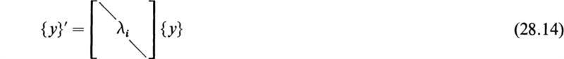
Substituting this relation into (28.8) and premultiplying by [M]–1 yields
Since [M] is the modal matrix of [A], the term [M]–1[A][M] is a diagonal matrix with the eigenvalues of [A] on the main diagonal:
The result is that the transformed system is uncoupled, that is, (28.14) may be represented by the single scalar differential equation
whose general solution is
where ck is an arbitrary constant. Returning to (28.14), the general solution may be written in the form
From (28.12) the general solution to (28.8) now becomes
From Sec. 20 the modal matrix is defined as
where {x}k is the kth eigenvector of [A]. Substituting (28.19) into (28.18) and expanding gives the general solution to (28.8) in terms of an eigenvector expansion:
This equation shows that the general solution may be expressed as a linear combination of the eigenvectors. By applying the initial conditions the n constants ck may be evaluated from (28.20):
where

and therefore
As an example of this method consider (28.1) subject to the initial conditions:
![]()
The matrix form of this equation is given in (28.5), and the initial condition vector is
The eigenvalues and eigenvectors of [A] are

Using (28.20), the general solution has the form
Applying (28.22) to determine the arbitrary constants yields

or

and the particular solution is
Since x1 = x, the solution to (28.1) is obtained from the first row of (28.25):
The only restriction on (28.20) is that the coefficient matrix must have distinct eigenvalues. Whenever multiple eigenvalues occur, a modified approach must be employed since all of the eigenvectors associated with the multiple root cannot be determined by usual methods. When this situation occurs, the alternate method is based on the method of undetermined coefficients.
For convenience, consider that the first eigenvalue of an nth-order system has a multiplicity of 3: that is, consider
where [A] is nth order and
![]()
To solve (28.27) assume a solution in the form†
Substituting this assumed solution into (28.27) gives
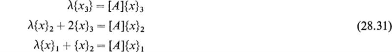
By employing the definition of eigenvectors and eigenvalues, the summations on each side of the equality may be canceled. The remaining expression becomes
Equating like powers of t yields
which may be solved sequentially for the three unknown eigenvectors.
Once the unknown eigenvectors have been evaluated, the general solution becomes
for which the n arbitrary constants may be evaluated in the usual manner by application of the initial conditions.
When the matrix [A] is a function of the independent variable t, the set of differential equations (28.7) may be integrated by means of the Peano-Baker method.† The principle of this method of integration is quite simple. Let the initial conditions of the system be such that
where {x0} is a column vector of initial values of the elements of {x}. Direct integration of (28.8) gives the following integral equation:
where t′ is a subsidiary variable of integration. This integral equation may be solved by repeated substitutions of {x} from the left-hand member of (29.2) into the integral. If the integral operator is introduced
then (29.2) may be written in the following form:
By repeated substitution, the following equation is obtained:
Let
This expression has been called the matrizant of [A]. In the series (29.6) [U] is the unit matrix of order n and the second term is the integral of [A] taken between the limits 0 and t. To obtain Q[A]Q[A], [A] and Q[A] are multiplied in the order [A] Q[A] and the product is integrated between 0 and t. The remaining terms are formed in the same manner. If the elements of the matrix [A(t)] remain bounded in the range 0 to t, it may be shown that the series (29.6) is absolutely and uniformly convergent and that it defines the square matrix G[A] in a unique manner.
The solution of the set of differential equations (28.8) is given by
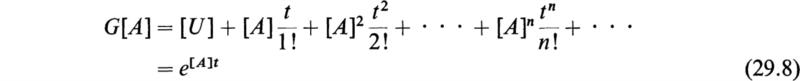
If the elements of the matrix [A] are constants, we have, by direct integration of the series (29.6),
Therefore, if [A] is a matrix of constants, the solution of (28.8) is
The interpretation of e[A]t, for purposes of calculation, may be made by the use of Sylvester’s theorem (24.2). To illustrate the general procedure, consider the second-order case in which the matrix [A] has the form
In this case the characteristic equation of [A] is given by
Let the two roots of (29.11) or the eigenvalues of (29.10) be given by
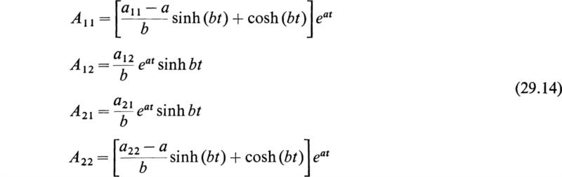
By the use of Sylvester’s theorem (24.2), the function may be expressed in the following form:
where
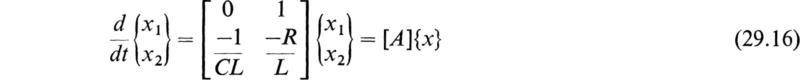
To illustrate this method of solution by an example of technical importance, consider the differential equations
These differential equations govern the oscillation of a series electric circuit having a resistance R, an inductance L, and a capacitance C, all in series (see Chap. 5). The variable q is the charge on the capacitance, and i is the current that flows in the circuit. The free oscillations of such a circuit are completely determined when the initial charge q0 and the initial current i0 of the circuit at t = 0 are specified. If we let x1=q and x2 = i, Eqs. (29.15) may be written in the standard matrix form:
The characteristic equation of [A] is, in this case,
In this case
The oscillations of the circuit are given by the following matrix equation:
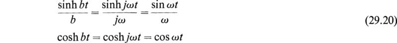
where the elements Aij are given by (29.14). If b is imaginary so that b =jω, then we have
so that the hyperbolic functions are replaced by trigonometric functions and the circuit oscillates. If b = 0, the circuit is critically damped and sinh(bt)/b becomes indeterminate. When this is evaluated by L’Hospital’s rule for indeterminate forms, it is seen that it must be replaced by t. The result (29.19) is thus seen to be a convenient expression that gives the current and charge of the circuit in terms of the initial conditions in concise form.
The Peano-Baker method is a convenient method for the integration of homogeneous linear differential equations with variable coefficients. As an example of the general procedure, consider the differential equation
This equation is known as Stokes’s equation in the mathematical literature of the diffraction and reflection of electromagnetic waves and in quantum mechanics.†
In order to reduce this equation to the form of (28.8), let
The system
replaces the original equation (29.21). Let the initial condition vector at t = 0 be
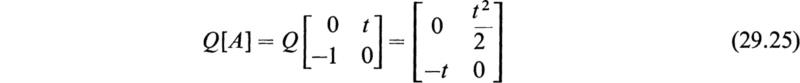
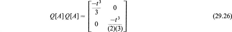
The matrizant G[A] is now computed by means of the series (29.6):
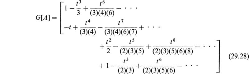
The first few terms of the matrizant are, by (29.6),
The elements of the matrizant G[A] are series expansions of the Bessel functions of order ![]() The solution of Stokes’s equation may be expressed in terms of the initial conditions in the form
The solution of Stokes’s equation may be expressed in terms of the initial conditions in the form
Besides the homogeneous first-order matrix differential equation considered in the last section, systems of nonhomogeneous equations are also of considerable interest. A typical equation of this type may be written in the following form:
where [A] = coefficient matrix
{f} = vector of forcing functions
{x} = unknown vector
As previously considered, both [A] and {f} may be functions of the independent variable.
The method of solving the system (30.1) presented in this section is the adjoint method. This method yields a solution to (30.1) by seeking a solution to the following set of adjoint equations:
where [Y] is an unknown matrix. The reasons for choosing the particular form for the adjoint system given in (30.2) will become clear as the process of solution unfolds.
The method proceeds as follows: premultiply (30.1) by [Y]′ and post-multiply the transpose of (30.2) by {x}. Adding the two resulting equations together yields
However, the two terms on the left are the derivative of a product and therefore (30.3) may be rewritten as
Integrating this equation between the limits of 0 and t and recalling that

gives
Hence, the solution to (30.1) is
where [Y] is the solution to the adjoint equation (30.2), which is homogeneous with convenient initial conditions.
If the coefficient matrix [A] is a constant matrix, the solution to (30.1) as given by (30.6) may be reduced to the following result:
As an example consider the equation
For this equation

Applying the method of Sec. 26 yields
Substituting this result into (30.11) gives
In this section we shall simply state the conditions required for the existence and uniqueness of solutions to matrix differential equations without showing the proof.
Before presenting these conditions further notation will be introduced in order to simplify the equations. Instead of writing the matrix differential equations as we have thus far, the following notation will be used:
where [L] = an operator matrix
{f} = a matrix of forcing functions
This notation may be used to represent (30.1) as follows:
![]()
Likewise (28.10) may be represented by (31.1) if
![]()
and
![]()
Hence any set of simultaneous differential equations may be written in the compact form of (31.1).
Besides (31.1) the corresponding homogeneous equation must be considered ; that is,
The conditions for the existence and uniqueness of a solution to (31.1) may be stated as follows:
1. A solution to (31.1) is unique if and only if the corresponding homogeneous equation (31.2) possesses only a trivial solution.
2. A solution to (31.1) exists† if and only if the vector {f} is orthogonal to all solutions of the homogeneous adjoint equation [L]′{x} = {0}.
The mathematical analysis of a considerable variety of physical problems leads to a formulation involving a differential equation that may be reduced to the following form:
where F(t) is a single-valued periodic function of fundamental period T. An equation of this type is known as Hill’s equation in the mathematical literature. If a change of variable of the form
is introduced into the Hill equation (32.1), the equation is transformed into
as a consequence of the periodicity of F(t). Hence Hill’s equation is invariant under the change of variable (32.2), and it is thus apparent that it is necessary only to obtain a solution of (32.1) in a fundamental interval ![]() The final values of y and
The final values of y and ![]() at the end of one interval of the variation of F(t) are the initial values of y and
at the end of one interval of the variation of F(t) are the initial values of y and ![]() in the following interval.
in the following interval.
Let u1(t) and u2(t) be two linearly independent solutions of Hill’s equation (32.1) in the fundamental interval ![]() Let y = x1 and
Let y = x1 and ![]() Then we have
Then we have
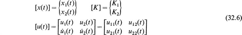
where K1 and K2 are arbitrary constants. Equations (32.4) may be written in the following convenient matrix form:
The following notation will be introduced in order to simplify the writing:
In this notation (32.5) may be expressed in the following concise form:
is called the Wronskian of the two solutions u1(t) and u2(t). It is a constant in the fundamental interval ![]() as may be shown by differentiation. Since the two solutions u1(t) and u2(t) are linearly independent, W0 ≠ 0. The matrix [u(t)] is therefore nonsingular and has the following inverse:
as may be shown by differentiation. Since the two solutions u1(t) and u2(t) are linearly independent, W0 ≠ 0. The matrix [u(t)] is therefore nonsingular and has the following inverse:
At t = 0, (32.7) reduces to
If this is premultiplied by [u(0)]–1, the result may be written in the following form:
This equation determines the column of arbitrary constants in terms of the initial conditions. If (32.11) is now substituted into (32.7), the result is
At the end of the fundamental interval, t = T, and the solution is given in terms of the initial conditions by the equation
Since, during the second fundamental interval, Hill’s equation has the same form as it has during the first interval, the relation expressing the initial and final values of [x(t)] in this interval has the same form as that given in (32.13). Therefore, at the end of the second cycle of the variation of F(t) we have
Introduce the following notation:
It is easy to see that, at the end of n periods of the variation of F(t), the solution of Hill’s equation is given by
and the solution within the (n + l)st interval is given by
This gives the solution of Hill’s equation at any time t > 0 in terms of the initial conditions and two linearly independent solutions in the fundamental interval ![]() The solution involves the computation of positive integral powers of the matrix [M].
The solution involves the computation of positive integral powers of the matrix [M].
As a consequence of the constancy of the Wronskian determinant W0 given by (32.8), the determinant of the matrix [M] is equal to unity. We thus have
The characteristic equation of [M] is
If A + D ≠ ±2, the eigenvalues of [M] are given by
and in this case [M] has distinct eigenvalues. By Sylvester’s theorem (24.2) the nth power of [M] may easily be computed. The result is
where
Equation (32.21) gives the proper form for [M]n only when A + D ≠ ±2. When A + D = ±2, the two eigenvalues of [M] are not distinct and a confluent form of Sylvester’s theorem must be used to compute [M]n.†
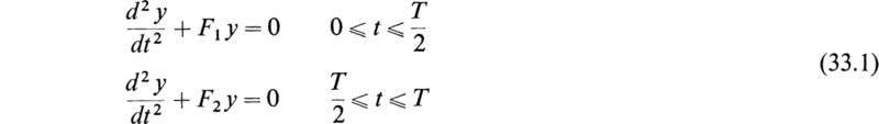
If the function F(t) has the form of the rectangular ripple of Fig. 33.1, Eq. (32.1) is known as the Hill-Meissner equation. The Hill-Meissner equation is of
Fig. 33.1
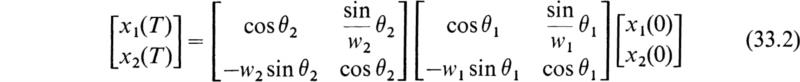
importance in the study of the oscillations of the driving rods of electric locomotives, and its solution is easily effected by the use of matrix algebra. In this case Eq. (32.1) reduces to two equations of the form
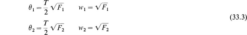
The solution of Eqs. (33.1) at t = T may be expressed in terms of the initial values of y and ![]() at t = 0 by the equation
at t = 0 by the equation
where ![]() and
and
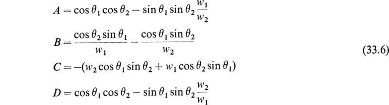
If the indicated matrix multiplication in (33.2) is performed, the result may be written in the following form:
In this case the matrix [M] has the form
where
The eigenvalues of [M] are given by
The values of y and ![]() after the end of n complete periods of the square-wave variation are given by
after the end of n complete periods of the square-wave variation are given by
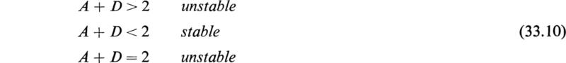
The nature of the solution of the Hill-Meissner equation depends on the form taken by the powers of the matrix [M], as given by (32.22). There are two separate cases to be considered. If A + D > 2, a must have a positive real part and the elements of [M]n increase exponentially with the number of periods, n. This leads to an unstable solution in physical applications. If, on the other hand, A + D < 2, a must be a pure imaginary number and the elements of [M]n oscillate with n. This leads to stable solutions in physical applications. The dividing line leads to the case A + D = 2. In this case the eigenvalues of [M] are repeated and both have the value μ1 = μ2 = 1. The form (32.22) is no longer applicable and must be replaced by one obtained from a confluent form of Sylvester’s theorem. In general the condition A + D = 2 leads to instability in physical problems. The question of stability may be summarized by the following expressions:
In any special cases the conditions for stability or instability may be deduced from (33.8).
The properties of matrices may be used to determine the roots of algebraic equations. As a simple example, consider the equation
Let the following third-order matrix be constructed:
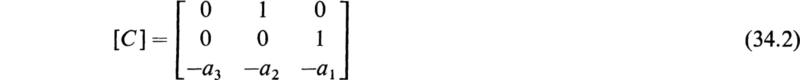
This matrix is called the companion matrix of the cubic equation (34.1). It is easy to show that the characteristic equation of the companion matrix [C] is the cubic equation. Therefore the eigenvalues of [C] are the roots of (34.1). The general algebraic equation of the nth degree
has a companion matrix of the nth order
The eigenvalues of [C], μ1, μ2, μ3,. . . , μn, are the roots of the equation (34.3). If the various roots of the nth-degree equation (34.3) are real and distinct and if μ1 is the root having the largest absolute value, then it can be shown by Sylvester’s theorem (24.2) that for a sufficiently large m we have
That is, for a sufficiently large-power m, a further multiplication of [C]m by [C] yields a new matrix whose elements are μ1 times the elements of [C]m. This multiple, μ1, is the dominant root of (34.3). A practical procedure for extracting the dominant root of an equation is to choose an arbitrary column vector of the nth order (x) and set up the following sequence:
Then, for a sufficiently large m, we have
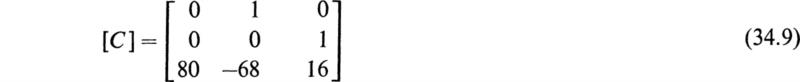
so that after a sufficient number of multiplications one more multiplication merely multiplies all the elements of the vector (x)m by a common factor. This common factor μ1 is the largest root of the equation and the largest eigenvalue of the companion matrix. As a simple numerical example, consider the following cubic equation:
The companion matrix of this equation
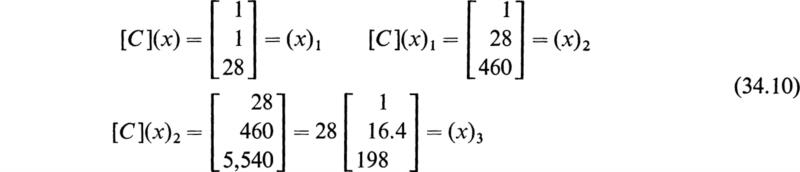
We now choose the arbitrary column vector

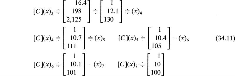
By direct multiplication we obtain
The factor 28 may be discarded since we are interested only in the ratios of similar elements after successive multiplication. Let ![]() denote the fact that a factor has been discarded, and proceed.
denote the fact that a factor has been discarded, and proceed.
Further multiplications only multiply the elements of the vectors by a factor of 10. Hence the dominant root is μ1 = 10. After having determined the dominant root, it may be divided out by dividing the polynomial f(z) = z3 – 16z2 + 68z – 80 by z – 10. This procedure may be performed by the synthetic division

Since the remainder is zero, the dominant root is exactly μ1 = 10. The polynomial f(z) is seen to have the factors f(z) = (z – 10)(z2 – 6z + 8). The roots of the quadratic z2 – 6z + 8 = 0 are μ2 = 4 and μ3 = 2. The eigenvalues of the companion matrix (34.9) are therefore μ1 = 10, μ2 = 4, μ3 = 2. If only the smallest root of the equation is desired, the substitution z=1/y may be made in Eq. (34.3) and the companion matrix of the resulting equation in y may be constructed. The iteration scheme (34.7) then yields the largest root in y and therefore the smallest root of the original equation.
The method of matrix iteration may be used to determine repeated and complex roots of algebraic equations.†
1. Solve the following system of equations by the use of determinants:

2. Evaluate the determinant

3. Solve the following system of equations:

4. Prove Cramer’s rule for the general case of n equations.
![]()
compute [a]10.

compute [a]–2.
7. Find the characteristic equation and the eigenvalues of the following matrix:

![]()
is transformed to the diagonal form
![]()
where Tθ is the following matrix:
![]()
and tan2θ = 2h/(a – b) (Jacobi’s transformation).

![]()
has properties similar to those of the imaginary number ![]() Show that [J]2 = –U, where U is the second-order unit matrix, and that [J]3 = –[J], [J]4 = U, [J]5 = [J], etc.
Show that [J]2 = –U, where U is the second-order unit matrix, and that [J]3 = –[J], [J]4 = U, [J]5 = [J], etc.
11. Determine the eigenvalues and eigenvectors of the matrix

12. Determine the roots of the equation z3 – 16z2 + 65z – 50 = 0 by the matrix iteration method.
13. Solve the differential equation d2y/dt2 + w2y = 0, subject to the conditions y(0) = y0 and ![]() by the Peano-Baker method.
by the Peano-Baker method.
14. Show that (18.1) is always consistent.
15. Using the matrix method illustrated in Sec. 18, solve (18.3) for x1 and x3 in terms of x2.
16. Find the value of the constant c for which the system

is consistent, and find the solution.
17. Derive (28.7).
18. Given (30.2) and (30.7), derive (30.8).
19. If [A] is a constant matrix, show that (30.10) reduces to (30.11).
20. If [A] is a diagonal matrix, show that f([A]) must equal [f(aii)]; for example,

21. Verify that (30.14) is the solution to (30.12).
22. Solve the following ([A] is the matrix in Prob. 7 above):

23. Solve the following systems:
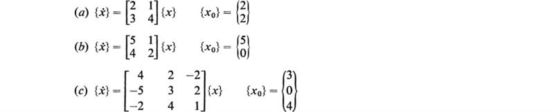
(Hochstadt, 1964)
24. Solve the following differential equations by reducing them to first-order matrix equations:

(Hochstadt, 1964)
25. Find the eigenvalues and eigenvectors of the following matrices:
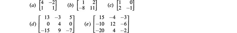
(Kreyszig, 1962)
1931. Bôcher, M.: “Introduction to Higher Algebra,” The Macmillan Company, New York.
1932. Turnbull, H. W., and A. C. Aitken: “An Introduction to the Theory of Canonical Matrices,” Blackie and Son, Ltd., Glasgow.
1937. Pipes, L. A.: Matrices in Engineering, Electrical Engineering, vol. 56, pp. 1177–1190.
1938. Frazer, R. A., W. J. Duncan, and A. R. Collar: “Elementary Matrices,” Cambridge University Press, New York.
1946. MacDuffee, C. C.: “The Theory of Matrices,” Chelsea Publishing Co., New York.
1949. Wedderburn, J. H. M.: “Lectures on Matrices,” J. W. Edwards, Publisher, Incorporated, Ann Arbor, Mich.
1950. Zurmuhl, R.: “Matrizen,” Springer-Verlag OHG, Berlin.
1951. Kaufmann, A., and M. Denis-Papin: “Cours de calcul matriciel,” Editions Albin Michel, Paris.
1953. Paige, L. J., and Olga Taussky (eds.): “Simultaneous Linear Equations and the Determination of Eigenvalues,” National Bureau of Standards, Applied Mathematics Series 29, August.
1956. Friedman, B.: “Principles and Techniques of Applied Mathematics,” John Wiley & Sons, Inc., New York.
1958. Hohn, F. E.: “Elementary Matrix Algebra,” The Macmillan Company, New York.
1960. Bellman, R.: “Introduction to Matrix Analysis,” McGraw-Hill Book Company, New York.
1962. Kreyszig, E.: “Advanced Engineering Mathematics,” John Wiley & Sons, Inc., New York.
1963. Pipes, L. A.: “Matrix Methods for Engineers,” Prentice-Hall, Inc., Englewood Cliffs, N.J.
1964. Hochstadt, H.: “Differential Equations,” Holt, Rinehart and Winston, Inc., New York.
† Rank may also be defined as the order of the largest nonvanishing minor contained in the matrix.
† For an excellent and thorough theoretical discussion of the subject of linear algebraic equations, see Hohn, 1958, chap. 5 (see References).
‡ Ibid, for a detailed proof.
§ See Hohn, 1958, chap. 5, for a detailed proof (see References).
† This restriction may be expanded to include multiple eigenvalues as long as there are n linear independent eigenvectors associated with [M].
‡ M. Bôcher, “Introduction to Higher Algebra,” The Macmillan Company, New York, 1931.
† M. Bôcher, “Introduction to Higher Algebra,” p. 296, The Macmillan Company, New York, 1931.
† H. Hotelling, New Methods in Matrix Calculation, The Annals of Mathematical Statistics, vol. 14, no. 1, pp. 1–34, March, 1943.
† G. E. Forsythe, Solving Linear Equations Can Be Interesting, Bulletin of the American Mathematical Society, vol. 59, no. 4, pp. 299–329, July, 1953.
† L. Fox, H. D. Huskey, and J. H. Wilkinson, Notes on the Solution of Algebraic Linear Simultaneous Equations, Quarterly Journal of Mechanics and Applied Mathematics, vol. 1, pp.149–173, 1948.
† R. A. Frazer, W. J. Duncan, and A. R. Collar, “Elementary Matrices,” pp. 78–79, Cambridge University Press, New York, 1938.
† Convergence is guaranteed provided S(μr) converges for each eigenvalue. Cf. Frazer, Duncan, and Collar, 1957, p. 81 (see References).
† Arbitrary constants have been omitted from the terms involving the unknown eigenvectors since at most an eigenvector is known up to an arbitrary constant.
† See E. L. Ince, “Ordinary Differential Equations,” pp. 408–415, Longmans, Green & Co., Ltd., London, 1927.
† See “Tables of the Modified Hankel Functions of Order One-third,” Harvard University Press, Cambridge, Mass., 1945.
† To be precise, the operator matrix must have a closed range. Cf. Friedman, 1956 (see References).
† See L. A. Pipes, Matrix Solutions of Equations of the Mathieu-Hill Type, Journal of Applied Physics, vol. 24, no. 7, pp. 902–910, July, 1953.
† See L. A. Pipes, Matrix Solution of Polynomial Equations, Journal of the Franklin Institute, vol. 225, no. 4, pp. 437–454, April, 1938.