2.1 Scalar, Vector, Matrix, and Tensor

From left to right, the graphic representations of a scalar, vector, matrix, and tensor
![$$\hat {S}^{[z]}$$](../images/489509_1_En_2_Chapter/489509_1_En_2_Chapter_TeX_IEq1.png) ) as
) as 

 a matrix with two indexes. Here, one can see that the difference between a (D × D) matrix and a D
2-component vector in our context is just the way of labeling the tensor elements. Transferring among vector, matrix, and tensor like this will be frequently used later. Graphically, we use a dot with two bonds to represent a matrix and its two indexes (Fig. 2.1).
a matrix with two indexes. Here, one can see that the difference between a (D × D) matrix and a D
2-component vector in our context is just the way of labeling the tensor elements. Transferring among vector, matrix, and tensor like this will be frequently used later. Graphically, we use a dot with two bonds to represent a matrix and its two indexes (Fig. 2.1).
In above, we use states of spin-1∕2 as examples, where each index can take two values. For a spin-S state, each index can take d = 2S + 1 values, with d called the bond dimension. Besides quantum states, operators can also be written as tensors. A spin-1∕2 operator  (α = x, y, z) is a (2 × 2) matrix by fixing the basis, where we have
  . In the same way, an N-spin operator can be written as a 2N-th order tensor, with Nbra and Nket indexes.3
We would like to stress some conventions about the “indexes” of a tensor (including matrix) and those of an operator. A tensor is just a group of numbers, where their indexes are defined as the labels labeling the elements. Here, we always put all indexes as the lower symbols, and the upper “indexes” of a tensor (if exist) are just a part of the symbol to distinguish different tensors. For an operator which is defined in a Hilbert space, it is represented by a hatted letter, and there will be no “true” indexes, meaning that both upper and lower “indexes” are just parts of the symbol to distinguish different operators.
2.2 Tensor Network and Tensor Network States
2.2.1 A Simple Example of Two Spins and Schmidt Decomposition

 .
.
The graphic representation of the Schmidt decomposition (singular value decomposition of a matrix). The positive-defined diagonal matrix λ, which gives the entanglement spectrum (Schmidt numbers), is defined on a virtual bond (dumb index) generated by the decomposition
Graphically, we have a small TN , where we use green squares to represent the unitary matrices U and V , and a red diamond to represent the diagonal matrix λ. There are two bonds in the graph shared by two objects, standing for the summations (contractions) of the two indexes in Eq. (2.4), a and a′. Unlike s (or s′), the space of the index a (or a′) is not from any physical Hilbert space. To distinguish these two kinds, we call the indexes like s the physical indexes and those like a the geometrical or virtual indexes. Meanwhile, since each physical index is only connected to one tensor, it is also called an open bond.
Some simple observations can be made from the Schmidt decomposition. Generally speaking, the index a (also a′ since λ is diagonal) contracted in a TN carry the quantum entanglement [4]. In quantum information sciences, entanglement is regarded as a quantum version of correlation [4], which is crucially important to understand the physical implications of TN. One usually uses the entanglement entropy to measure the strength of the entanglement, which is defined as  . Since the state should be normalized, we have
  . For
. For  , obviously |ψ〉 = λ
1|u〉1|v〉1 is a product state with zero entanglement S = 0 between the two spins. For
, obviously |ψ〉 = λ
1|u〉1|v〉1 is a product state with zero entanglement S = 0 between the two spins. For  , the entanglement entropy
  , where S takes its maximum if and only if λ
1 = ⋯ = λ
χ. In other words, the dimension of a geometrical index determines the upper bound of the entanglement.
, where S takes its maximum if and only if λ
1 = ⋯ = λ
χ. In other words, the dimension of a geometrical index determines the upper bound of the entanglement.
 matrix C′ (
 ) that minimizes the norm


2.2.2 Matrix Product State
![$$\displaystyle \begin{aligned} \begin{array}{rcl} C_{s_1 \cdots s_{N-1}s_N} = \sum_{a_{N-1}} C^{[N-1]}_{s_1 \cdots s_{N-1},a_{N-1}} A^{[N]}_{s_{N}, a_{N-1} }. \end{array} \end{aligned} $$](../images/489509_1_En_2_Chapter/489509_1_En_2_Chapter_TeX_Equ8.png)
![$$\displaystyle \begin{aligned} \begin{array}{rcl} C_{s_1 \cdots s_{N-1} a_{N-1}} = \sum_{a_{N-2}} C^{[N-2]}_{s_1 \cdots s_{N-2},a_{N-2}} A^{[N-1]}_{s_{N-1}, a_{N-2} a_{N-1}}. \end{array} \end{aligned} $$](../images/489509_1_En_2_Chapter/489509_1_En_2_Chapter_TeX_Equ9.png)
![$$\displaystyle \begin{aligned} \begin{array}{rcl} C_{s_1 \cdots s_{N-1}s_N} = \sum_{a_{N-2} a_{N-1}} C^{[N-2]}_{s_1 \cdots s_{N-2},a_{N-2}} A^{[N-1]}_{s_{N-1}, a_{N-2} a_{N-1}} A^{[N]}_{s_{N}, a_{N-1}}. \end{array} \end{aligned} $$](../images/489509_1_En_2_Chapter/489509_1_En_2_Chapter_TeX_Equ10.png)
![$$\displaystyle \begin{aligned} \begin{array}{rcl} C_{s_1 \cdots s_{N-1}s_N} = \sum_{a_{1} \cdots a_{N-1}} A^{[1]}_{s_1, a_{1}} A^{[2]}_{s_2, a_{1} a_{2}} \cdots A^{[N-1]}_{s_{N-1}, a_{N-2} a_{N-1}} A^{[N]}_{s_{N}, a_{N-1}}. {} \end{array} \end{aligned} $$](../images/489509_1_En_2_Chapter/489509_1_En_2_Chapter_TeX_Equ11.png)
![$$\displaystyle \begin{aligned} \begin{array}{rcl} C_{s_1 \cdots s_{N-1}s_N} = \sum_{a_{1} \cdots a_{N}} A^{[1]}_{s_1, a_{N} a_{1}} A^{[2]}_{s_2, a_{1} a_{2}} \cdots A^{[N-1]}_{s_{N-1}, a_{N-2} a_{N-1}} A^{[N]}_{s_{N}, a_{N-1} a_{N}}, {} \end{array} \end{aligned} $$](../images/489509_1_En_2_Chapter/489509_1_En_2_Chapter_TeX_Equ12.png)

An impractical way to obtain an MPS from a many-body wave-function is to repetitively use the SVD

The graphic representations of the matrix product states with open (left) and periodic (right) boundary conditions
MPS is an efficient representation of a many-body quantum state. For a N-spin state, the number of the coefficients is 2N which increases exponentially with N. For an MPS given by Eq. (2.12), it is easy to count that the total number of the elements of all tensors is Ndχ 2 which increases only linearly with N. The above way of obtaining MPS with decompositions is also known as tensor train decomposition (TTD) in MLA , and MPS is also called tensor-train form [6]. The main aim of TTD is investigating the algorithms to obtain the optimal tensor-train form of a given tensor, so that the number of parameters can be reduced with well-controlled errors.
In physics, the above procedure shows that any states can be written in an MPS , as long as we do not limit the dimensions of the geometrical indexes. However, it is extremely impractical and inefficient, since in principle, the dimensions of the geometrical indexes {a} increase exponentially with N. In the following sections, we will directly applying the mathematic form of the MPS without considering the above procedure.
![$$\displaystyle \begin{aligned} \begin{array}{rcl} |\psi \rangle =tTr A^{[1]} A^{[2]} \cdots A^{[N]} |s_1s_2 \cdots s_N \rangle = tTr \prod_{n=1}^{N} A^{[n]} |s_n \rangle. {} \end{array} \end{aligned} $$](../images/489509_1_En_2_Chapter/489509_1_En_2_Chapter_TeX_Equ13.png)
2.2.3 Affleck–Kennedy–Lieb–Tasaki State

One possible configuration of the sparse anti-ferromagnetic ordered state. A dot represents the S = 0 state. Without looking at all the S = 0 states, the spins are arranged in the anti-ferromagnetic way
![$$\displaystyle \begin{aligned} \begin{array}{rcl} \hat{H}=\sum_n\left[\frac{1}{2} \hat{S}_n\cdot \hat{S}_{n+1}+\frac{1}{6} (\hat{S}_n\cdot \hat{S}_{n+1})^2+\frac{1}{3}\right]. {} \end{array} \end{aligned} $$](../images/489509_1_En_2_Chapter/489509_1_En_2_Chapter_TeX_Equ14.png)
 that projects the neighboring spins to the subspace of S = 2, Eq. (2.14) can be rewritten in the summation of projectors as
 with a zero energy.


![$$\displaystyle \begin{aligned} \begin{array}{rcl} \sigma^+ = \left[ {\begin{array}{*{30}c} 0 \quad 1 \\ 0 \quad 0 \\ \end{array}} \right], \quad \ \ \sigma^{z} = \left[ {\begin{array}{*{30}c} 1 \quad 0 \\ 0 \ \ -1 \\ \end{array}} \right], \quad \ \ \sigma^- = \left[ {\begin{array}{*{30}c} 0 \quad 0 \\ 1 \quad 0 \\ \end{array}} \right]. \quad \ \ {} \end{array} \end{aligned} $$](../images/489509_1_En_2_Chapter/489509_1_En_2_Chapter_TeX_Equ19.png)


An intuitive graphic representation of the AKLT
state. The big circles representing S = 1 spins, and the small ones are effective  spins. Each pair of spin-1∕2 connecting by a red bond forms a singlet state. The two “free” spin-1∕2 on the boundary give the edge state

![$$\displaystyle \begin{aligned} \begin{array}{rcl} I = \left[ {\begin{array}{*{30}c} 1 \quad 0 \\ 0 \quad 1 \\ \end{array}} \right]. {} \end{array} \end{aligned} $$](../images/489509_1_En_2_Chapter/489509_1_En_2_Chapter_TeX_Equ22.png)
 in the AKLT Hamiltonian is always acted on a singlet, then we have
  .
.2.2.4 Tree Tensor Network State (TTNS) and Projected Entangled Pair State (PEPS)
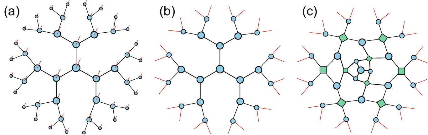
The illustration of (a) and (b) two different TTNSs and (c) MERA

(a) An intuitive picture of the projected entangled pair state. The physical spins (big circles) are projected to the virtual ones (small circles), which form the maximally entangled states (red bonds). (b)–(d) Three kinds of frequently used PEPSs
![$$\displaystyle \begin{aligned} \begin{array}{rcl} |\varPsi\rangle = tTr \prod_{n} P^{[n]} |s_n\rangle, {} \end{array} \end{aligned} $$](../images/489509_1_En_2_Chapter/489509_1_En_2_Chapter_TeX_Equ23.png)
Such a generalization makes a lot of senses in physics. One key factor regards the area law of entanglement entropy [12–17] which we will talk about later in this chapter. In the following as two straightforward examples, we show that PEPS can indeed represents non-trivial physical states including nearest-neighbor resonating valence bond (RVB) and Z 2spin liquid states. Note these two types of states on trees can be similarly defined by the corresponding TTNS.
2.2.5 PEPS Can Represent Non-trivial Many-Body States: Examples
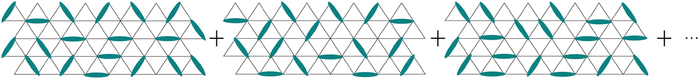
The nearest-neighbor RVB state is the superposition of all possible configurations of nearest-neighbor singlets


After the contraction of all geometrical indexes, the state is the superposition of all possible configurations consisting of nearest-neighbor dimers. This iPEPS looks different from the one given in Eq. (2.23) but they are essentially the same, because one can contract the B’s into P’s so that the PEPS is only formed by tensors defined on the sites.


2.2.6 Tensor Network Operators
![$$\displaystyle \begin{aligned} \begin{array}{rcl} \hat{O} = \sum_{\{s,a\}} \prod_n W_{s_n s_n^{\prime}, a_n a_{n+1}}^{[n]}|s_n\rangle \langle s_n^{\prime}|. {} \end{array} \end{aligned} $$](../images/489509_1_En_2_Chapter/489509_1_En_2_Chapter_TeX_Equ30.png)
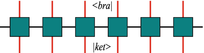
The graphic representation of a matrix product operator, where the upward and downward indexes represent the bra and ket space, respectively
![$$W^{[n]}_{::,00}=C^{[n]}$$](../images/489509_1_En_2_Chapter/489509_1_En_2_Chapter_TeX_IEq19.png) ,
, ![$$W^{[n]}_{::,01}=B^{[n]}$$](../images/489509_1_En_2_Chapter/489509_1_En_2_Chapter_TeX_IEq20.png) , and
, and ![$$W^{[n]}_{::,11}=A^{[n]}$$](../images/489509_1_En_2_Chapter/489509_1_En_2_Chapter_TeX_IEq21.png) with A
[n], B
[n], and C
[n] some d × d square matrices. We can write W
[n] in a more explicit 2 × 2 block-wise form as
with A
[n], B
[n], and C
[n] some d × d square matrices. We can write W
[n] in a more explicit 2 × 2 block-wise form as ![$$\displaystyle \begin{aligned} \begin{array}{rcl} W^{[n]}= \begin{pmatrix} C^{[n]} &\displaystyle 0 \\ B^{[n]} &\displaystyle A^{[n]} \end{pmatrix}. \end{array} \end{aligned} $$](../images/489509_1_En_2_Chapter/489509_1_En_2_Chapter_TeX_Equ31.png)
![$$\displaystyle \begin{aligned} \begin{array}{rcl} O &\displaystyle =&\displaystyle \sum_{n=1}^N A^{[1]} \otimes \cdots \otimes A^{[n-1]} \otimes B^{[n]} \otimes C^{[n+1]} \otimes \cdots \otimes C^{[N]} \\ &\displaystyle =&\displaystyle \sum_{n=1}^N \prod_{\otimes i=1}^{n-1} A^{[i]} \otimes B^{[n]} \otimes \prod_{\otimes j=n+1}^{N} C^{[j]}, {} \end{array} \end{aligned} $$](../images/489509_1_En_2_Chapter/489509_1_En_2_Chapter_TeX_Equ32.png)

The graphic representation of a projected entangled pair operator, where the upward and downward indexes represent the bra and ket space, respectively
![$$\displaystyle \begin{aligned} \begin{array}{rcl} W^{[n]}= \begin{pmatrix} I &\displaystyle 0 \\ X^{[n]} &\displaystyle I \end{pmatrix}, \end{array} \end{aligned} $$](../images/489509_1_En_2_Chapter/489509_1_En_2_Chapter_TeX_Equ33.png)
![$$\displaystyle \begin{aligned} \begin{array}{rcl} W^{[n]}= \begin{pmatrix} I &\displaystyle 0 &\displaystyle 0 \\ Z^{[n]} &\displaystyle 0 &\displaystyle 0 \\ X^{[n]} &\displaystyle Y^{[n]} &\displaystyle I \end{pmatrix}. \end{array} \end{aligned} $$](../images/489509_1_En_2_Chapter/489509_1_En_2_Chapter_TeX_Equ34.png)
![$$\displaystyle \begin{aligned} \begin{array}{rcl} W^{[1]}= \begin{pmatrix} I &\displaystyle 0 &\displaystyle 0 \end{pmatrix}, \ \ \end{array} \end{aligned} $$](../images/489509_1_En_2_Chapter/489509_1_En_2_Chapter_TeX_Equ35.png)
![$$\displaystyle \begin{aligned} \begin{array}{rcl} W^{[N]}= \begin{pmatrix} 0 \\ 0 \\ I \end{pmatrix}. \end{array} \end{aligned} $$](../images/489509_1_En_2_Chapter/489509_1_En_2_Chapter_TeX_Equ36.png)

![$$\displaystyle \begin{aligned} \begin{array}{rcl} W^{[n]}= \begin{pmatrix} I &\displaystyle 0 &\displaystyle 0 \\ \hat{S}^z &\displaystyle 0 &\displaystyle 0 \\ h \hat{S}^x &\displaystyle \hat{S}^z &\displaystyle I \end{pmatrix}. \end{array} \end{aligned} $$](../images/489509_1_En_2_Chapter/489509_1_En_2_Chapter_TeX_Equ38.png)
 . The Fourier transformation is written as
 (
( ) the annihilation (creation) operator on the n-th site. The MPO representation of such a Fourier transformation is given by
 the identical operator in the corresponding Hilbert space.
The MPO formulation also allows for a convenient and efficient representation of the Hamiltonians with longer range interactions [54]. The geometrical bond dimensions will in principle increase with the interaction length. Surprisingly, a small dimension is needed to approximate the Hamiltonian with long-range interactions that decay polynomially [46].
Besides, MPO can be used to represent the time evolution operator  with Trotter–Suzuki decomposition, where τ is a small positive number called Trotter–Suzuki step [55, 56]. Such an MPO is very useful in calculating real, imaginary, or even complex time evolutions, which we will present later in detail. An MPO can also give a mixed state.
![$$\displaystyle \begin{aligned} \begin{array}{rcl} \hat{O} = \sum_{\{s,a\}} \prod_n W_{s_n s_n^{\prime}, a_n^1 a_n^2 a_n^3 a_n^4}^{[n]} |s_n\rangle \langle s_n^{\prime}|. {} \end{array} \end{aligned} $$](../images/489509_1_En_2_Chapter/489509_1_En_2_Chapter_TeX_Equ41.png)
2.2.7 Tensor Network for Quantum Circuits

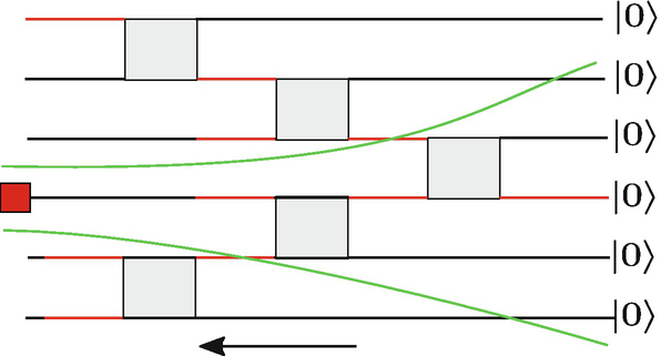
The TN representation of a quantum circuit. Two-body unitaries act on a product state of a given number of constituents |0〉⊗⋯ ⊗|0〉 and transform it into a target entangled state |ψ〉
 , where i, i + 1 label the neighboring constituents of a one-dimensional system. The evolution operator for a time t is
  , and can be decomposed into a sequence of infinitesimal time evolution steps [58] (more details will be given in Sect. 3.1.3)

 and τ = t∕N. This is obviously a quantum circuit made by two-qubit gates with depth N. Conversely, any quantum circuit naturally possesses an arrow of time, it transforms a product state into an entangled state after a sequence of two-body gates.
 with
with  the rest part of the system besides A.
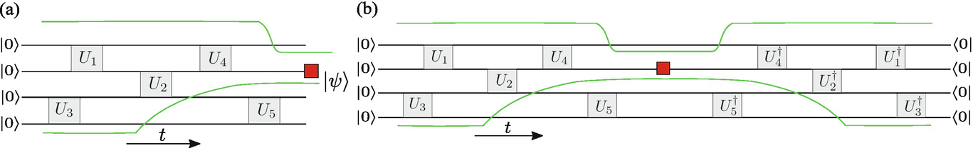
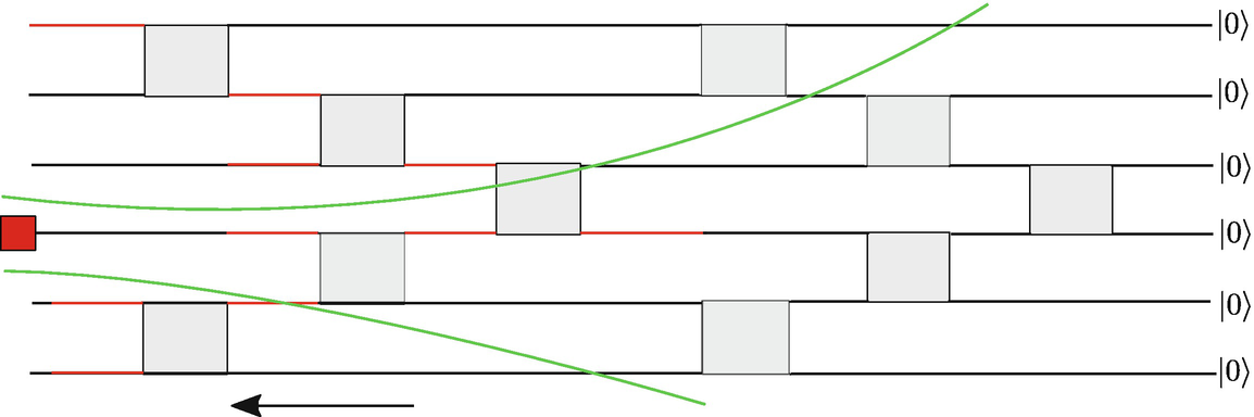
(a) The past casual cone of the red site. The unitary gate U
5 does not affect the reduced density matrix of the red site. This is verified by computing explicitly ρ
A by tracing over all the others constituents. (b) In the TN of ρ
A, U
5 is contracted with  , which gives an identity
The TN of the reduced density matrix is formed by a set of unitaries that define the past causal cone of the region A (see the area between the green lines in Fig. 2.13). The rest unitaries (for instance, the  and its conjugate in the right sub-figure of Fig. 2.13) will be eliminated in the TN of the reduced density matrix. The contraction of the causal cone can thus be rephrased in terms of the multiplication of a set of transfer matrices, each performing the computation from t to t − 1. The maximal width of these transfer matrices defines the width of the causal cone, which can be used as a good measure of the complexity of computing ρ
A [59]. The best computational strategy one can find to compute exactly ρ
A will indeed always scale exponentially with the width of the cone [57].
and its conjugate in the right sub-figure of Fig. 2.13) will be eliminated in the TN of the reduced density matrix. The contraction of the causal cone can thus be rephrased in terms of the multiplication of a set of transfer matrices, each performing the computation from t to t − 1. The maximal width of these transfer matrices defines the width of the causal cone, which can be used as a good measure of the complexity of computing ρ
A [59]. The best computational strategy one can find to compute exactly ρ
A will indeed always scale exponentially with the width of the cone [57].

The MPS as a quantum circuit. Time flows from right to left so that the lowest constituent is the first to interact with the auxiliary D-level system. Here we show the past causal cone of a single constituent. Similarly, the past causal cone of A made by adjacent constituent has the same form starting from the upper boundary of A
Using the gauge degrees of freedom of an MPS, we can modify its past causal cone structure to make its region as small as possible, in such a way decreasing the computational complexity of the actual computation of specific ρ A. A convenient choice is the center gauge used in iDMRG
Again, the gauge degrees of freedom can be used to modify the structure of the past causal cone of a certain spin. As an example, the iDMRG center gauge is represented in Fig. 2.15.
The width of the causal cone increases as we increase the depth of the quantum circuit generating the MPS state
2.3 Tensor Networks that Can Be Contracted Exactly
2.3.1 Definition of Exactly Contractible Tensor Network States
The notion of the past causal cone can be used to classify TNSs based on the complexity of computing their contractions. It is important to remember that the complexity strongly depends on the object that we want to compute, not just the TN. For example, the complexity of an MPS for a N-qubit state scales only linearly with N. However, to compute the n-site reduced density matrix, the cost scales exponentially with n since the matrix itself is an exponentially large object. Here we consider to compute scalar quantities, such as the observables of one- and two-site operators.
We define the a TNS to be exactly contractible when it is allowed to compute their contractions with a cost that is a polynomial to the elementary tensor dimensions D. A more rigorous definition can be given in terms of their tree width see, e.g., [57]. From the discussion of the previous section, it is clear that such a TNS corresponds to a bounded causal cone for the reduced density matrix of a local subregion. In order to show this, we now focus on the cost of computing the expectation value of local operators and their correlation functions on a few examples of TNSs .
The relevant objects are thus the reduced density matrix of a region A made of a few consecutive spins, and the reduced density matrix of two disjoint blocks A
1 and A
2 of which each made of a few consecutive spins. Once we have the reduced density matrices of such regions, we can compute arbitrary expectation values of local operators by  and
and  with
with  ,
,  ,
,  arbitrary operators defined on the regions A, A
1, A
2.
arbitrary operators defined on the regions A, A
1, A
2.
2.3.2 MPS Wave-Functions

The MPS wave-function representation in left-canonical form

The expectation value of a single-site operator with an MPS wave-function
Two-point correlation function of an MPS wave-function
2.3.3 Tree Tensor Network Wave-Functions
An alternative kind of wave-functions are the TTNSs [63–69]. In a TTNS, one can add the physical bond on each of the tensor, and use it as a many-body state defined on a Caley-tree lattice [63]. Here, we will focus on the TTNS with physical bonds only on the outer leafs of the tree.

A binary TTNS made of several layers of third-order tensors. Different layers are identified with different colors. The arrows flow in the opposite direction of the time while being interpreted as a quantum circuit

The expectation value of a local operator of a TTNS . We see that after applying the isometric properties of the tensors, the past causal cone of a single site has a bounded width. The calculation again boils down to a calculation of transfer matrices. This time the transfer matrices evolve between different layers of the tree

The computation of the correlation function of two operators separated by a given distance boils down to the computation of a certain power of transfer matrices. The computation of the casual cone can be simplified in a sequential way, as depicted in the last two sub-figures
2.3.4 MERA Wave-Functions

The TN of MERA . The MERA has a hierarchical structure consisting of several layers of disentanglers and isometries. The computational time flows from the center towards the edge radially, when considering MERA as a quantum circuit. The unitary and isometric tensors and the network geometry are chosen in order to guarantee that the width of the causal cone is bounded

Past causal cone of a single-site operator for a MERA

Two-point correlation function in the MERA
As in the case of the TTNS , we can indeed perform the explicit calculation of the past causal cone of a single-site operator (Fig. 2.24). There we show the TN contraction of the required expectation value, and then simplify it by taking into account the contractions of the unitary and isometric tensors outside the casual cone with a bounded width involving at most four auxiliary constituents.
The calculation of a two-point correlation function of local operators follows a similar idea and leads to the contraction shown in Fig. 2.25. Once more, we see that the computation of the two-point correlation function can be done exactly due to the bounded width of the corresponding casual cone.
2.3.5 Sequentially Generated PEPS Wave-Functions
The MERA and TTNS can be generalized to two-dimensional lattices [64, 74]. The generalization of MPS to 2D, on the other hand, gives rise to PEPS . In general, it belongs to the 2D TNs that cannot be exactly contracted [24, 78].

(a) A sequentially generated PEPS. All tensors but the central one (green in the figure) are isometries, from the in-going bonds (marked with ingoing arrows) to the outgoing ones. The central tensor represents a normalized vector on the Hilbert space constructed by the physical Hilbert space and the four copies of auxiliary spaces, one for each of its legs. (b) The norm of such PEPS, after implementing the isometric constraints, boils down to the norm of its central tensor

(a) The reduced density matrices of a PEPS that is sequentially generated containing two consecutive spins (one of them is the central spin. (b) The reduced density matrix of a local region far from the central site is generally hard to compute, since it can give rise to an arbitrarily large causal cone. For the reduced density matrix of any of the corners with a L × L PEPS, which is the most consuming case, it leads to a causal cone with a width up to L∕2. That means the computation is exponentially expensive with the size of the system
Differently from MPS, the causal cone of a PEPS cannot be transformed by performing a gauge transformation. However, as firstly observed by F. Cucchietti (private communication), one can try to approximate a PEPS of a given causal cone with another one of a different causal cone, by, for example, moving the center site. This is not an exact operation, and the approximations involved in such a transformation need to be addressed numerically. The systematic study of the effect of these approximations has been studied recently in [80, 81]. In general, we have to say that the contraction of a PEPS wave-function can only be performed exactly with exponential resources. Therefore, efficient approximate contraction schemes are necessary to deal with PEPS.
2.3.6 Exactly Contractible Tensor Networks
We have considered above, from the perspective of quantum circuits, whether a TNS can be contracted exactly by the width of the casual cones. Below, we reconsider this issue from the aspect of TN.
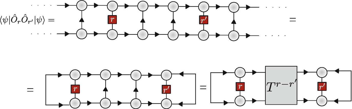
If one starts with contracting an arbitrary bond, there will be a tensor with six bonds. As the contraction goes on, the number of bonds increases linearly with the boundary ∂ of the contracted area, thus the memory increases exponentially as O(χ ∂) with χ the bond dimension
![$$\displaystyle \begin{aligned} \begin{array}{rcl} Z = \sum_{\{a\}} \prod_{n=1}^{N_L} \prod_{m=1}^{M_n} T^{[n,m]}_{a_{n,m,1},a_{n,m,2},a_{n,m,3}} \prod_k v^{[k]}_{a_k}, \end{array} \end{aligned} $$](../images/489509_1_En_2_Chapter/489509_1_En_2_Chapter_TeX_Equ44.png)
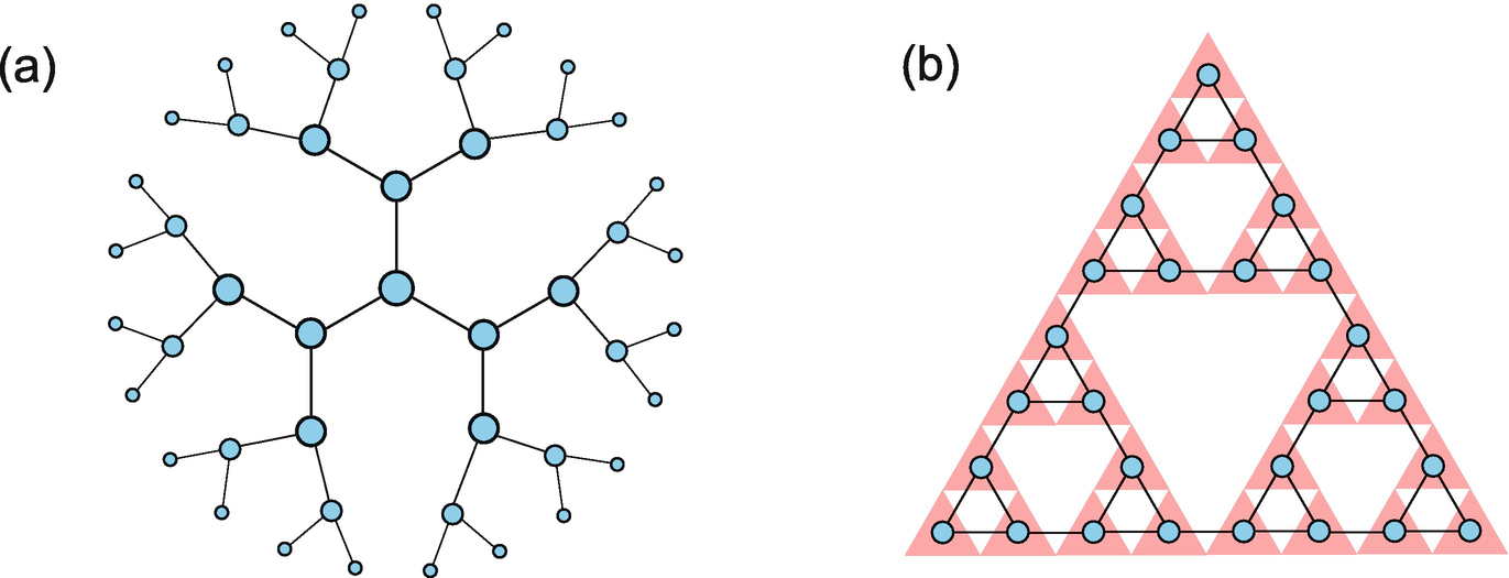
Two kinds of TNs that can be exactly contracted: (a) tree and (b) fractal TNs. In (b), the shadow shows the Sierpiński gasket, where the tensors are defined in the triangles
![$$\displaystyle \begin{aligned} \begin{array}{rcl} v_{a_3}^{\prime} = \sum_{a_1a_2} T^{[N_L m]}_{a_1a_2a_3} v^{[k_1]}_{a_1} v^{[k_2]}_{a_2}. \end{array} \end{aligned} $$](../images/489509_1_En_2_Chapter/489509_1_En_2_Chapter_TeX_Equ45.png)
We can see from the above contraction that if the graph does not contain any loops, i.e., has a tree-like structure, the dimensions of the obtained tensors during the contraction will not increase unboundedly. Therefore, the TN defined on it can be exactly contracted. This is again related to the area law of entanglement entropy that a loop-free TN satisfies: to separate a tree-like TN into two disconnecting parts, the number of bonds that needs to be cut is only one. Thus, the upper bond of the entanglement entropy between these two parts is constant, determined by the dimension of the bond that is cut. This is also consistent with the analyses based on the maximal width of the casual cones.
Another example that can be exactly contracted is the TN defined on the fractal called Sierpiński gasket (Fig. 2.29b) (see, e.g., [82, 83]). The TN can represent the partition function of the statistical model defined on the Sierpiński gasket, such as Ising and Potts model. As explained in Sec. II, the tensor is given by the probability distribution of the three spins in a triangle.

The third example is called algebraically contractible TNs [84, 85]. The tensors that form the TN possess some special algebraic properties, so that even the bond dimensions increase after each contraction, the rank of the bonds is kept unchanged. It means one can introduce some projectors to lower the bond dimension without causing any errors.

For a square TN of an arbitrary size formed by the fourth-order Is, obviously we have its contraction Z = d with d the bond dimension. The reason is that the contraction is the summation of only d non-zero values (each equals to 1).


The fusion rule of the copy tensor: the contraction of two copy tensors of N 1-th and N 2-th order gives a copy tensor of (N 1 + N 2 − N)-th order, with N the number of the contracted bonds


 with N
T the total number of tensors.
with N
T the total number of tensors.
2.4 Some Discussions
2.4.1 General Form of Tensor Network
![$$\displaystyle \begin{aligned} \begin{array}{rcl} \mathscr{T}_{\{s\}} = \sum_{\{a\}} \prod_{n} T^{[n]}_{s^n_1s^n_2 \cdots,a^n_1 a^n_2 \cdots}. {} \end{array} \end{aligned} $$](../images/489509_1_En_2_Chapter/489509_1_En_2_Chapter_TeX_Equ52.png)
 -th order tensor, with
  the total number of the open indexes {s}.
Each tensor in the TN can possess different number of open or geometrical indexes. For an MPS , each tensor has one open index (called physical bond) and two geometrical indexes; for PEPS on square lattice, it has one open and four geometrical indexes. For the generalizations of operators, the number of open indexes is two for each tensor. It also allows hierarchical structure of the TN, such as TTNS and MERA .
![$$\displaystyle \begin{aligned} \begin{array}{rcl} Z = \sum_{\{a\}} \prod_{n} T^{[n]}_{a^n_1 a^n_2 \cdots}. {} \end{array} \end{aligned} $$](../images/489509_1_En_2_Chapter/489509_1_En_2_Chapter_TeX_Equ53.png)
 or
or  , where Z can be the cost function (e.g., energy or fidelity) to be maximized or minimized. The TN contraction algorithms mainly deal with the scalar TNs.
2.4.2 Gauge Degrees of Freedom
For a given state, its TN
representation is not unique. Let us take translational invariant MPS as an example. One may insert a (full-rank) matrix U and its inverse U
−1 on each of the virtual bonds and then contracted them, respectively, into the two neighboring tensors. The tensors of new MPS
become ![$$\tilde {A}^{[n]}_{s, a a'} = \sum _{bb'} U_{ab} A^{[n]}_{s, b b'} U^{-1}_{a' b'}$$](../images/489509_1_En_2_Chapter/489509_1_En_2_Chapter_TeX_IEq47.png) . In fact, we only put an identity I = UU
−1, thus do not implement any changes to the MPS. However, the tensors that form the MPS change, meaning the TN representation changes. It is also the case when inserting an matrix and its inverse on any of the virtual bonds of a TN state, which changes the tensors without changing the state itself. Such degrees of freedom is known as the gauge degrees of freedom, and the transformations are called gauge transformations.
. In fact, we only put an identity I = UU
−1, thus do not implement any changes to the MPS. However, the tensors that form the MPS change, meaning the TN representation changes. It is also the case when inserting an matrix and its inverse on any of the virtual bonds of a TN state, which changes the tensors without changing the state itself. Such degrees of freedom is known as the gauge degrees of freedom, and the transformations are called gauge transformations.
The gauge degrees of on the one hand may cause instability to TN simulations. Algorithms for finite and infinite PEPS were proposed to fix the gauge to reach higher stability [86–88]. On the other hand, one may use gauge transformation to transform a TN state to a special form, so that, for instance, one can implement truncations of local basis while minimizing the error non-locally [45, 89] (we will go back to this issue later). Moreover, gauge transformation is closely related to other theoretical properties such as the global symmetry of TN states, which has been used to derive more compact TN representations [90], and to classify many-body phases [91, 92] and to characterize non-conventional orders [93, 94], just to name a few.
2.4.3 Tensor Network and Quantum Entanglement
The numerical methods based on TN face great challenges, primarily that the dimension of the Hilbert space increases exponentially with the size. Such an “exponential wall” has been treated in different ways by many numeric algorithms, including the DFT methods [95] and QMC approaches [96].
The power of TN has been understood in the sense of quantum entanglement: the entanglement structure of low-lying energy states can be efficiently encoded in TNSs . It takes advantage of the fact that not all quantum states in the total Hilbert space of a many-body system are equally relevant to the low-energy or low-temperature physics. It has been found that the low-lying eigenstates of a gapped Hamiltonian with local interactions obey the area law of the entanglement entropy [97].
 of the system, its reduced density matrix is defined as
  , with
  denotes the spatial complement of
  . The entanglement entropy is defined as

 the size of the boundary. In particular, for a D-dimensional system, one has
 is obtained when tracing out the block B, i.e.,
  (see Fig. 2.32). In the limit of large distance between A and C blocks with l
AC ≫ ξ
corr, one has the reduced density matrix satisfying
(see Fig. 2.32). In the limit of large distance between A and C blocks with l
AC ≫ ξ
corr, one has the reduced density matrix satisfying 
 that has no correlations between A and C; here B
l and B
r sit at the two ends of the block B, which together span the original block.
that has no correlations between A and C; here B
l and B
r sit at the two ends of the block B, which together span the original block.
Bipartition of a 1D system into two half chains. Significant quantum correlations in gapped ground states occur only on short length scales
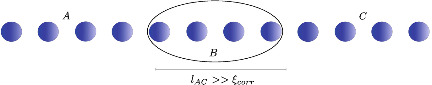
To argue the 1D area law, the chain is separated into three subsystems denoted by A, B, and C. If the correlation length ξ
corr is much larger than the size of B (denoted by l
AC), the reduced density matrix by tracing B approximately satisfies 
 on the block B that completely disentangles the left from the right part as
 implies that there exists a tensor
  with 0 ≤ a, a′, s ≤ χ − 1 and basis {|ψ
A〉}, {|ψ
B〉}, {|ψ
C〉} defined on the Hilbert spaces belonging to A, B, C such that
with 0 ≤ a, a′, s ≤ χ − 1 and basis {|ψ
A〉}, {|ψ
B〉}, {|ψ
C〉} defined on the Hilbert spaces belonging to A, B, C such that 
This argument directly leads to the MPS description and gives a strong hint that the ground states of a gapped Hamiltonian is well represented by an MPS of finite bond dimensions, where B in Eq. (2.59) is analog to the tensor in an MPS. Let us remark that every state of N spins has an exact MPS representation if we allow χ to grow exponentially with the number of spins [102]. The whole point of MPS is that a ground state can typically be represented by an MPS where the dimension χ is small and scales at most polynomially with the number of spins: this is the reason why MPS-based methods are more efficient than exact diagonalization.
For the 2D PEPS
, it is more difficult to strictly justify the area law of entanglement entropy. However, we can make some sense of it from the following aspects. One is the fact that PEPS can exactly represent some non-trivial 2D states that satisfies the area law, such as the nearest-neighbor RVB and Z2 spin liquid mentioned above. Another is to count the dimension of the geometrical bonds  between two subsystems, from which the entanglement entropy satisfies an upper bound as
  .10
.10
 satisfies
  , and the upper bound of the entanglement entropy fulfills the area law given by Eq. (2.56), which is

Open Access This chapter is licensed under the terms of the Creative Commons Attribution 4.0 International License (http://creativecommons.org/licenses/by/4.0/), which permits use, sharing, adaptation, distribution and reproduction in any medium or format, as long as you give appropriate credit to the original author(s) and the source, provide a link to the Creative Commons license and indicate if changes were made.
The images or other third party material in this chapter are included in the chapter's Creative Commons license, unless indicated otherwise in a credit line to the material. If material is not included in the chapter's Creative Commons license and your intended use is not permitted by statutory regulation or exceeds the permitted use, you will need to obtain permission directly from the copyright holder.