6.1 Motivation and General Ideas
An impression one may have for the TN approaches of the quantum lattice models is that the algorithm (i.e., how to contract and/or truncate) will dramatically change when considering different models or lattices. This motivates us to look for more unified approaches. Considering that a huge number of problems can be transformed to TN contractions, one general question we may ask is: how can we reduce a non-deterministic polynomial hard TN contraction problem approximately to an effective one that can be computed exactly and efficiently by classical computers? We shall put some principles while considering this question: the effective problem should be as simple as possible, containing as few parameters to solve as possible. We would like to coin this principle for TN contractions as the ab initio optimization principle (AOP) of TN [1]. The term “ab inito” is taken here to pay respect to the famous ab inito principle approaches in condensed matter physics and quantum chemistry (see several recent reviews in [2–4]). Here, “ab inito” means to think from the very beginning, with least prior knowledge of or assumptions to the problems.
One progress achieved in the spirit of AOP is the TRD introduced in Sect. 5.4. Considering the TN on an infinite square lattice, its contraction is reduced to a set of self-consistent eigenvalue equations that can be efficiently solved by classical computers. The variational parameters are just two tensors. One advantage of TRD is that it connects the TN algorithms (iDMRG , iTEBD , CTMRG ), which are previously considered to be quite different, in a unified picture.
Another progress made in the AOP spirit is called QES for simulating infinite-size physical models [1, 5, 6]. It is less dependent on the specific models; it also provides a natural way for designing quantum simulators and for hybridized-quantum-classical simulations of many-body systems. Hopefully in the future when people are able to readily realize the designed Hamiltonians on artificial quantum platforms, QES will enable us to design the Hamiltonians that will realize quantum many-body phenomena.
6.2 Simulating One-Dimensional Quantum Lattice Models
Let us firstly take the ground-state simulation of the infinite-size 1D quantum system as an example. The Hamiltonian is the summation of two-body nearest-neighbor terms, which reads  . The translational invariance is imposed. The first step is to choose a supercell (e.g., a finite part of the chain with
  sites). Then the Hamiltonian of the supercell is
  , and the Hamiltonian connecting the supercell to the rest part is
  (note the interactions are nearest neighbor).
 as
as 
 , we equivalently chose to shift
  for algorithmic consideration. The errors of these two ways concerning the ground state are at the same level (
 ). Introduce an ancillary index a and rewrite
  as a sum of operators as
 and
and  are two sets of one-body operators (labeled by a) acting on the left and right one of the two spins (s and s′) associated with
  , respectively (Fig. 6.1). Equation (6.2) can be easily achieved directly from the Hamiltonian or using eigenvalue decomposition. For example, for the Heisenberg interaction with
  with
with  the spin operators. We have
  with
with  ,
,  ,
,  (α = x, y, z), hence we can define
  and
and  .
.
 , with
  representing the physical spins inside the supercell, as
 .
.  and
and  act on the first and last sites of the supercell, respectively. One can see that
  represents a set of operators labeled by two indexes (a′ and a) that act on the supercell.
 in the local basis (
 ) is a fourth-order cell tensor (Fig. 6.1) as
 as
as  . With the cell tensor T, the ground-state properties can be solved using the TN algorithms (e.g., TRD) introduced above. The ground state is given by the MPS given by Eq. (5.59).
 by using
  as the coefficients
 is the effective Hamiltonian in iDMRG
[9–11] or the methods which represent the RG
of Hilbert space by MPS
[12, 13]. The indexes {b} are considered as virtual spins with basis {|b〉}. The virtual spins are called the entanglement bath sites in the QES
.
is the effective Hamiltonian in iDMRG
[9–11] or the methods which represent the RG
of Hilbert space by MPS
[12, 13]. The indexes {b} are considered as virtual spins with basis {|b〉}. The virtual spins are called the entanglement bath sites in the QES
.
 and
and  locate on the boundaries of
  , whose coefficients satisfy
 and
and  are just two-body Hamiltonians, of which each acts on the bath site and its neighboring physical site on the boundary of the bulk; they define the infinite boundary condition for simulating the time evolution of 1D quantum systems [14].
 and
and  can also be written in a shifted form as


 is independent on τ, called the physical-bath Hamiltonian. Then
  can be written as the shift of a few-body Hamiltonian as
  , where
  has the standard summation form as
 and
and  with the bath dimension χ, the coefficient matrix of
  is (2χ × 2χ). Then
  can be generally expanded by
  with
with  the generators of the SU(χ) group, and define the magnetic field and coupling constants associated to the entanglement bath
 denoting the SU(χ) spin operators and
  the operators of the physical spin (with the identity included).
 just gives the Hamiltonian between two spin-1∕2’s. Thus, it can be expanded by the spin (or Pauli) operators
  as
as 
 ,
,  ,
,  , and
, and  . Then with α
1 ≠ 0 and α
2 ≠ 0, we have
. Then with α
1 ≠ 0 and α
2 ≠ 0, we have  as the coupling constants, and
  and
and  the magnetic fields on the first and second sites, respectively.
  only provides a constant shift of the Hamiltonian which does not change the eigenstates.
 and
and  for the infinite quantum Ising chain in a transverse field [18]. The original Hamiltonian reads
  , and
, and  and
and  satisfies
 coupling and a vertical field emerge in
  and
and  . This is interesting, because the
  interaction is the stabilizer on the open boundaries of the cluster state, a highly entangled state that has been widely used in quantum information sciences [19, 20]. More relations with the cluster state are to be further explored.
 (denoted by |Ψ(Sb
1b
2)〉) by tracing over the entanglement-bath degrees of freedom. To this aim, we calculate the reduced density matrix of the bulk as
(denoted by |Ψ(Sb
1b
2)〉) by tracing over the entanglement-bath degrees of freedom. To this aim, we calculate the reduced density matrix of the bulk as 
 with
with  the eigenvector of Eq. (6.5) or (5.57). It is easy to see that
  is the central tensor in the central-orthogonal MPS
(Eq. (5.59)), thus the
is the central tensor in the central-orthogonal MPS
(Eq. (5.59)), thus the  is actually the reduced density matrix of the MPS. Since the MPS optimally gives the ground state of the infinite model, therefore,
  of the few-body ground state optimally gives the reduced density matrix of the original model.
In Eq. (6.12), the summation of the physical interactions is within the supercell that we choose to construct the cell tensor. To improve the accuracy to, e.g., capture longer correlations inside the bulk, one just needs to increase the supercell in  . In other words,
  and
and  are obtained by TRD
from the supercell of a tolerable size
are obtained by TRD
from the supercell of a tolerable size  , and
, and  is constructed with a larger bulk as
  with
with  . Though
  becomes more expensive to solve, we have many well-established finite-size algorithms to compute its dominant eigenvector. We will show below that this way is extremely useful in higher dimensions.
6.3 Simulating Higher-Dimensional Quantum Systems
For (D > 1)-dimensional quantum systems on, e.g., square lattice, one can use different update schemes to calculate the ground state. Here, we explain an alternative way by generalizing the above 1D simulation to higher dimensions [5]. The idea is to optimize the physical-bath Hamiltonians by the zero-loop approximation (simple update, see Sect. 5.3), e.g., iDMRG
on tree lattices [21, 22], and then construct the few-body Hamiltonian  with larger bulks. The loops inside the bulk will be fully considered when solving the ground state of
  , thus the precision will be significantly improved compared with the zero-loop approximation.
 , and the interaction between two neighboring supercells is the same, i.e.,
  . By shifting
  , we define
  and decompose it as
 and
and  are two sets of operators labeled by a that act on the two spins (s and s′) in the supercell, respectively (see the texts below Eq. (6.2) for more detail).
 and
and  (Fig. 6.3) as
 . The cell tensor that defines the TN
is given by the coefficients of
. The cell tensor that defines the TN
is given by the coefficients of  as
as 
 , which is a PEPO
defined on a square lattice. Infinite layers of the PEPO
, which is a PEPO
defined on a square lattice. Infinite layers of the PEPO  give the cubic TN
.
give the cubic TN
.
Graphical representation of the cell tensor for 2D quantum systems (Eq. (6.18))
 that is defined on the Bethe lattice. The cell tensor is defined exactly in the same way as Eq. (6.19). With the Bethe approximation, there are five variational tensors, which are Ψ (central tensor) and v
[x] (x = 1, 2, 3, 4, boundary tensors). Meanwhile, we have five self-consistent equations that encodes the 3D TN
that is defined on the Bethe lattice. The cell tensor is defined exactly in the same way as Eq. (6.19). With the Bethe approximation, there are five variational tensors, which are Ψ (central tensor) and v
[x] (x = 1, 2, 3, 4, boundary tensors). Meanwhile, we have five self-consistent equations that encodes the 3D TN  , which are given by five matrices as
 ![$$\displaystyle \begin{aligned} \begin{array}{rcl} \mathscr{H}_{S'b_1^{\prime}b_2^{\prime}b_3^{\prime}b_4^{\prime},Sb_1b_2b_3b_4} = \sum_{a_1a_2a_3a_4} T_{S'Sa_1a_2a_3a_4} v^{[1]}_{a_1b_1 b_1^{\prime}} v^{[2]}_{a_2b_2 b_2^{\prime}} v^{[3]}_{a_3b_3 b_3^{\prime}} v^{[4]}_{a_4b_4 b_4^{\prime}}, {}\\ \end{array} \end{aligned} $$](../images/489509_1_En_6_Chapter/489509_1_En_6_Chapter_TeX_Equ20.png)
![$$\displaystyle \begin{aligned} \begin{array}{rcl} M^{[1]}_{a_1b_1b_1^{\prime},a_3b_3b_3^{\prime}} = \sum_{S'Sa_2a_4b_2b_2^{\prime}b_4b_4^{\prime}} T_{S'Sa_1a_2a_3a_4} A^{[1]\ast}_{S'b_1^{\prime}b_2^{\prime}b_3^{\prime}b_4^{\prime}} v^{[2]}_{a_2b_2 b_2^{\prime}} A^{[1]}_{Sb_1b_2b_3b_4} v^{[4]}_{a_4b_4 b_4^{\prime}},{}\\ \end{array} \end{aligned} $$](../images/489509_1_En_6_Chapter/489509_1_En_6_Chapter_TeX_Equ21.png)
![$$\displaystyle \begin{aligned} \begin{array}{rcl} M^{[2]}_{a_2b_2b_2^{\prime},a_4b_4b_4^{\prime}} = \sum_{S'Sa_1a_3b_1b_1^{\prime}b_3b_3^{\prime}} T_{S'Sa_1a_2a_3a_4} A^{[2]\ast}_{S'b_1^{\prime}b_2^{\prime}b_3^{\prime}b_4^{\prime}} v^{[1]}_{a_1b_1 b_1^{\prime}} A^{[2]}_{Sb_1b_2b_3b_4} v^{[3]}_{a_3b_3 b_3^{\prime}},{}\\ \end{array} \end{aligned} $$](../images/489509_1_En_6_Chapter/489509_1_En_6_Chapter_TeX_Equ22.png)
![$$\displaystyle \begin{aligned} \begin{array}{rcl} M^{[3]}_{a_1b_1b_1^{\prime},a_3b_3b_3^{\prime}} = \sum_{S'Sa_2a_4b_2b_2^{\prime}b_4b_4^{\prime}} T_{S'Sa_1a_2a_3a_4} A^{[3]\ast}_{S'b_1^{\prime}b_2^{\prime}b_3^{\prime}b_4^{\prime}} v^{[2]}_{a_2b_2 b_2^{\prime}} A^{[3]}_{Sb_1b_2b_3b_4} v^{[4]}_{a_4b_4 b_4^{\prime}},{}\\ \end{array} \end{aligned} $$](../images/489509_1_En_6_Chapter/489509_1_En_6_Chapter_TeX_Equ23.png)
![$$\displaystyle \begin{aligned} \begin{array}{rcl} M^{[4]}_{a_2b_2b_2^{\prime},a_4b_4b_4^{\prime}} = \sum_{S'Sa_1a_3b_1b_1^{\prime}b_3b_3^{\prime}} T_{S'Sa_1a_2a_3a_4} A^{[4]\ast}_{S'b_1^{\prime}b_2^{\prime}b_3^{\prime}b_4^{\prime}} v^{[1]}_{a_1b_1 b_1^{\prime}} A^{[4]}_{Sb_1b_2b_3b_4} v^{[3]}_{a_3b_3 b_3^{\prime}}.{}\\ \end{array} \end{aligned} $$](../images/489509_1_En_6_Chapter/489509_1_En_6_Chapter_TeX_Equ24.png)
![$$\displaystyle \begin{aligned} \begin{array}{rcl} \varPsi_{Sb_1b_2b_3b_4} = \sum_{b} A^{[2]}_{Sb_1bb_3b_4} R^{[2]}_{b b_2}. {} \end{array} \end{aligned} $$](../images/489509_1_En_6_Chapter/489509_1_En_6_Chapter_TeX_Equ25.png)
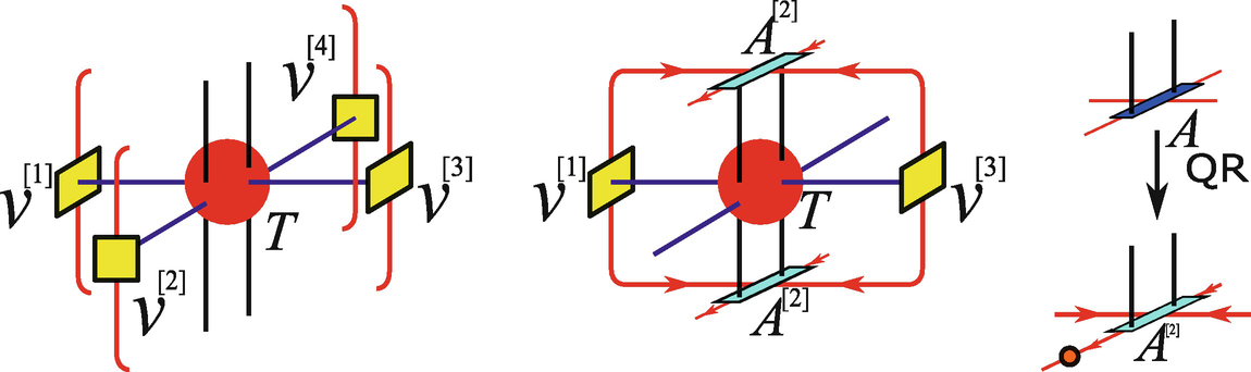
The left figure is the graphic representations of  in Eq. (6.20), and we take Eq. (6.22) from the self-consistent equations as an example shown in the middle. The QR
decomposition in Eq. (6.25) is shown in the right figure, where the arrows indicate the direction of orthogonality of A
[3] in Eq. (6.26)
in Eq. (6.20), and we take Eq. (6.22) from the self-consistent equations as an example shown in the middle. The QR
decomposition in Eq. (6.25) is shown in the right figure, where the arrows indicate the direction of orthogonality of A
[3] in Eq. (6.26)
![$$\displaystyle \begin{aligned} \begin{array}{rcl} \sum_{Sb_1 b_3 b_4} A^{[2] \ast}_{Sb_1bb_3b_4} A^{[2]}_{Sb_1b'b_3b_4} = I_{bb'}. {} \end{array} \end{aligned} $$](../images/489509_1_En_6_Chapter/489509_1_En_6_Chapter_TeX_Equ26.png)
The self-consistent equations can be solved recursively. By solving the leading eigenvector of  given by Eq. (6.20), we update the central tensor Ψ. Then according to Eq. (6.25), we decompose Ψ to obtain A
[x], then update M
[x] in Eqs. (6.21)–(6.24), and update each v
[x] by M
[x]v
[x]. Repeat this process until all the five variational tensors converge. The algorithm is the generalized DMRG
based on infinite tree PEPS
[21, 22]. Each boundary tensor can be understood as the infinite environment of a tree branch, thus the original model is actually approximated at this stage by that defined on an Bethe lattice. Note that when only looking at the tree locally (from one site and its nearest neighbors), it looks the same to the original lattice. Thus, the loss of information is mainly long range, i.e., from the destruction of loops.
given by Eq. (6.20), we update the central tensor Ψ. Then according to Eq. (6.25), we decompose Ψ to obtain A
[x], then update M
[x] in Eqs. (6.21)–(6.24), and update each v
[x] by M
[x]v
[x]. Repeat this process until all the five variational tensors converge. The algorithm is the generalized DMRG
based on infinite tree PEPS
[21, 22]. Each boundary tensor can be understood as the infinite environment of a tree branch, thus the original model is actually approximated at this stage by that defined on an Bethe lattice. Note that when only looking at the tree locally (from one site and its nearest neighbors), it looks the same to the original lattice. Thus, the loss of information is mainly long range, i.e., from the destruction of loops.
 with
with  the PEPO
of the Bethe model and
the PEPO
of the Bethe model and  a tree iPEPS
(Fig. 6.5). To see this, let us start with the local contraction (Fig. 6.5a) as
a tree iPEPS
(Fig. 6.5). To see this, let us start with the local contraction (Fig. 6.5a) as ![$$\displaystyle \begin{aligned} \begin{array}{rcl} Z_{Bethe} = \sum \varPsi^{\ast}_{S'b_1^{\prime}b_2^{\prime}b_3^{\prime}b_4^{\prime}} \varPsi_{Sb_1b_2b_3b_4} T_{S'Sa_1a_2a_3a_4} v^{[1]}_{a_1b_1 b_1^{\prime}} v^{[2]}_{a_2b_2 b_2^{\prime}} v^{[3]}_{a_3b_3 b_3^{\prime}} v^{[4]}_{a_4b_4 b_4^{\prime}}.\qquad {} \end{array} \end{aligned} $$](../images/489509_1_En_6_Chapter/489509_1_En_6_Chapter_TeX_Equ27.png)
 satisfied,
  is the ground state of
  .
.
The left figure shows the local contraction that encodes the infinite TN
for simulating the 2D ground state. By substituting with the self-consistent equations, the TN representing  can be reconstructed, with
  the tree PEPO
of the Bethe model and
the tree PEPO
of the Bethe model and  a PEPS
Now, we constrain the growth so that the TN
covers the infinite square lattice. Inevitably, some v
[x]s will gather at the same site. The tensor product of these v
[x]s in fact gives the optimal rank-1 approximation of the “correct” full-rank tensor here (Sect. 5.3.3). Suppose that one uses the full-rank tensor to replace its rank-1 version (the tensor product of four v
[x]’s), one will have the PEPO
of  (with H the Hamiltonian on square lattice), and the tree iPEPS
becomes the iPEPS defined on the square lattice. Compared with the NCD
scheme that employs rank-1 decomposition explicitly to solve TN contraction, one difference here for updating iPEPS is that the “correct” tensor to be decomposed by rank-1 decomposition contains the variational tensor, thus is in fact unknown before the equations are solved. For this reason, we cannot use rank-1 decomposition directly. Another difference is that the constraint, i.e., the normalization of the tree iPEPS, should be fulfilled. By utilizing the iDMRG
algorithm with the tree iPEPS, the rank-1 tensor is obtained without knowing the “correct” tensor, and meanwhile the constraints are satisfied. The zero-loop approximation of the ground state is thus given by the tree iPEPS.
(with H the Hamiltonian on square lattice), and the tree iPEPS
becomes the iPEPS defined on the square lattice. Compared with the NCD
scheme that employs rank-1 decomposition explicitly to solve TN contraction, one difference here for updating iPEPS is that the “correct” tensor to be decomposed by rank-1 decomposition contains the variational tensor, thus is in fact unknown before the equations are solved. For this reason, we cannot use rank-1 decomposition directly. Another difference is that the constraint, i.e., the normalization of the tree iPEPS, should be fulfilled. By utilizing the iDMRG
algorithm with the tree iPEPS, the rank-1 tensor is obtained without knowing the “correct” tensor, and meanwhile the constraints are satisfied. The zero-loop approximation of the ground state is thus given by the tree iPEPS.
![$$\displaystyle \begin{aligned} \begin{array}{rcl} \hat{\mathscr{H}} = \prod_{\langle n \in cluster, \alpha \in bath \rangle} \hat{\mathscr{H}}_{\partial}(n,\alpha) \prod_{\langle i,j \rangle \in cluster} [I-\tau \hat{H}(s_i,s_j)]. {} \end{array} \end{aligned} $$](../images/489509_1_En_6_Chapter/489509_1_En_6_Chapter_TeX_Equ28.png)
 is defined as the physical-bath Hamiltonian between the α-th bath site and the neighboring n-th physical site, and it is obtained by the corresponding boundary tensor v
[x(α)] and
is defined as the physical-bath Hamiltonian between the α-th bath site and the neighboring n-th physical site, and it is obtained by the corresponding boundary tensor v
[x(α)] and  (Fig. 6.6) as
 ![$$\displaystyle \begin{aligned} \begin{array}{rcl} \langle b_{\alpha}^{\prime}s_n^{\prime}| \hat{\mathscr{H}}_{\partial}(n,\alpha) |b_{\alpha}s_n\rangle = \sum_{a} v^{[x(\alpha)]}_{ab_{\alpha}^{\prime} b_{\alpha}} \langle s_n^{\prime} |\hat{F}_{L(R)}(s_n)_{a} | s_n\rangle. {} \end{array} \end{aligned} $$](../images/489509_1_En_6_Chapter/489509_1_En_6_Chapter_TeX_Equ29.png)
 is the operator defined in Eq. (6.17), and
 ![$$v^{[x(\alpha )]}_{ab_{\alpha }^{\prime } b_{\alpha }}$$](../images/489509_1_En_6_Chapter/489509_1_En_6_Chapter_TeX_IEq117.png) are the solutions of the SEEs
given in Eqs. (6.20)–(6.24).
are the solutions of the SEEs
given in Eqs. (6.20)–(6.24).
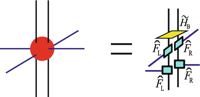
The left figure shows the few-body Hamiltonian  in Eq. (6.28). The middle one shows the physical-bath Hamiltonian
  that gives the interaction between the corresponding physical and bath site. The right one illustrates the state ansatz for the infinite system. Note that the boundary of the cluster should be surrounded by
  ’s, and each
  corresponds to an infinite tree brunch in the state ansatz. For simplicity, we only illustrate four of the
  s and the corresponding brunches
 in Eq. (6.28) can also be rewritten as the shift of a few-body Hamiltonian
  , i.e.,
  . We have
  possessing the standard summation form as
 . This equations gives a general form of the few-body Hamiltonian: the first term contains all the physical interactions inside the cluster, and the second contains all physical-bath interactions
  .
.  can be solved by any finite-size algorithms, such as exact diagonalization, QMC
, DMRG
[9, 23, 24], or finite-size PEPS
[25–27] algorithms. The error from the rank-1 decomposition will be reduced since the loops inside the cluster will be fully considered.
can be solved by any finite-size algorithms, such as exact diagonalization, QMC
, DMRG
[9, 23, 24], or finite-size PEPS
[25–27] algorithms. The error from the rank-1 decomposition will be reduced since the loops inside the cluster will be fully considered. after tracing over the entanglement-bath degrees of freedom. We have
  (with |Φ〉 the ground state of the infinite model) that well approximate by
 the coefficients of the ground state of
  .
.Figure 6.6 illustrates the ground state ansatz behind the few-body model. The cluster in the center is entangled with the surrounding infinite tree brunches through the entanglement-bath degrees of freedom. Note that solving Eq. (6.20) in Stage one is equivalent to solving Eq. (6.28) by choose the cluster as one supercell.
Some benchmark results of simulating 2D and 3D spin models can be found in Ref. [5]. For the ground state of Heisenberg model on honeycomb lattice, results of the magnetization and bond energy show that the few-body model of 18 physical and 12 bath sites suffers only a small finite-effect of O(10−3). For the ground state of 3D Heisenberg model on cubic lattice, the discrepancy of the energy per site is O(10−3) between the few-body model of 8 physical plus 24 bath sites and the model of 1000 sites by QMC . The quantum phase transition of the quantum Ising model on cubic lattice can also be accurately captured by such a few-body model, including determining the critical field and the critical exponent of the magnetization.
6.4 Quantum Entanglement Simulation by Tensor Network: Summary

The “ab initio optimization principle” to simulate quantum many-body systems
As to the classical computations, one will have a high flexibility to balance between the computational complexity and accuracy, according to the required precision and the computational resources at hand. On the one hand, thanks to the zero-loop approximation, one can avoid the conventional finite-size effects faced by the previous exact diagonalization, QMC , or DMRG algorithms with the standard finite-size models. In the QES , the size of the few-body model is finite, but the actual size is infinite as the size of the defective TN (see Sect. 5.3.3). The approximation is that the loops beyond the supercell are destroyed in the manner of the rank-1 approximation, so that the TN can be computed efficiently by classical computation. On the other hand, the error from the destruction of the loops can be reduced in the second stage by considering a cluster larger than the supercell. It is important that the second stage would introduce no improvement if no larger loops were contained in the enlarged cluster. From this point of view, we have no “finite-size” but “finite-loop” effects. In addition, this “loop” scheme explains why we can flexibly change the size of the cluster in stage two: which is just to restore the rank-1 tensors inside the chosen cluster with the full tensors.
 can be written as a linear combination of spin operators (and identity). Thus in this case, v
[x] simply plays the role of a classical mean field. If one only uses the bath calculation of the first stage to obtain the ground-state properties, the algorithm will be reduced to the zero-loop schemes such as tree DMRG
and simple update of iPEPS
. By choosing a large cluster and dim(b) = 1, the DMRG simulation in stage two becomes equivalent to the standard DMRG for solving the cluster in a mean field. By taking proper supercell, cluster, algorithms, and other computational parameters, the QES
approach can outperform others.
can be written as a linear combination of spin operators (and identity). Thus in this case, v
[x] simply plays the role of a classical mean field. If one only uses the bath calculation of the first stage to obtain the ground-state properties, the algorithm will be reduced to the zero-loop schemes such as tree DMRG
and simple update of iPEPS
. By choosing a large cluster and dim(b) = 1, the DMRG simulation in stage two becomes equivalent to the standard DMRG for solving the cluster in a mean field. By taking proper supercell, cluster, algorithms, and other computational parameters, the QES
approach can outperform others.
Relations to the algorithms (PEPS, DMRG, and ED) for the ground-state simulations of 2D and 3D Hamiltonian. The corresponding computational set-ups in the first (bath calculation) and second (solving the few-body Hamiltonian) stages are given above and under the arrows, respectively. Reused from [5] with permission
The QES approach with classical computations can be categorized as a cluster update scheme (see Sect. 4.3) in the sense of classical computations. Compared with the “traditional” cluster update schemes [26, 28–30], there exist some essential differences. The “traditional” cluster update schemes use the super-orthogonal spectra to approximate the environment of the iPEPS. The central idea of QES is different, which is to give an effective finite-size Hamiltonian; the environment is mimicked by the physical-bath Hamiltonians instead of some spectra.
In addition, it is possible to use full update in the first stage to optimize the interactions related to the entanglement bath. For example, one may use TRD
(iDMRG
, iTEBD
, or CTMRG
) to compute the environment tensors, instead of the zero-loop schemes. This idea has not been realized yet, but it can be foreseen that the interactions among the bath sites will appear in  . Surely the computation will become much more expensive. It is not clear yet how the performance would be.
The effective models under several bath-related methods: density functional theory (DFT , also known as the ab initio calculations), dynamical mean-field theory (DMFT) , and QES
Methods | DFT | DMFT | QES |
Effective models | Tight binding model | Single impurity model | Interacting few-body model |
The QES
allow for quantum simulations of infinite-size many-body systems by realizing the few-body models on the quantum platforms. There are several unique advantages. The first one concerns the size. One of the main challenges to build a quantum simulator is to access a large size. In this scheme, a few-body model of only O(10) sites already shows a high accuracy with the error ∼O(10−3) [1, 5]. Such sizes are accessible by the current platforms. Secondly, the interactions in the few-body model are simple. The bulk just contains the interactions of the original physical model. The physical-bath interactions are only two-body and nearest neighbor. But there exist several challenges. Firstly, the physical-bath interaction for simulating, e.g., spin-1∕2 models, is between a spin-1∕2 and a higher spin. This may require the realization of the interactions between SU(N) spins, which is difficult but possible with current experimental techniques [32–35]. The second challenge concerns the non-standard form in the physical-bath interaction, such as the  coupling in
  for simulating quantum Ising chain [see Eq. (6.15)] [18]. With the experimental realization of the few-body models, the numerical simulations of many-body systems will not only be useful to study natural materials. It would become possible to firstly study the many-body phenomena by numerics, and then realize, control, and even utilize these many-body phenomena in the bulk of small quantum devices.

 the density matrix of the QES
at the temperature T and Trbath the trace over the degrees of freedom of the bath sites.
the density matrix of the QES
at the temperature T and Trbath the trace over the degrees of freedom of the bath sites.  mimics the reduced density matrix of infinite-size system that traces over everything except the bulk. This idea has been used to simulate the quantum models in one, two, and three dimensions. The QES shows good accuracy at all temperatures, where relatively large error appears near the critical/crossover temperature.
One can readily check the consistency with the ground-state QES
. When the ground state is unique, the density matrix is defined as  with |Ψ〉 the ground state of the QES. In this case, Eqs. (6.32) and (6.16) are equivalent. With degenerate ground states, the equivalence should still hold when the spontaneous symmetry breaking occurs. With the symmetry preserved, it is an open question how the ground-state degeneracy affects the QES, where at zero temperature we have
  with {|Ψ
a〉} the degenerate ground states and
with {|Ψ
a〉} the degenerate ground states and  the degeneracy.

Open Access This chapter is licensed under the terms of the Creative Commons Attribution 4.0 International License (http://creativecommons.org/licenses/by/4.0/), which permits use, sharing, adaptation, distribution and reproduction in any medium or format, as long as you give appropriate credit to the original author(s) and the source, provide a link to the Creative Commons license and indicate if changes were made.
The images or other third party material in this chapter are included in the chapter's Creative Commons license, unless indicated otherwise in a credit line to the material. If material is not included in the chapter's Creative Commons license and your intended use is not permitted by statutory regulation or exceeds the permitted use, you will need to obtain permission directly from the copyright holder.