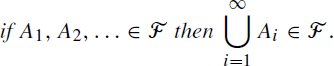
Summary. The very basic principles and tools of probability theory are set out. An event involving randomness may be described in mathematical terms as a probability space. Following an account of the properties of probability spaces, the concept of conditional probability is explained, and also that of the independence of events. There are many worked examples of calculations of probabilities.

1.1 Experiments with chance

Many actions have outcomes which are largely unpredictable in advance—tossing a coin and throwing a dart are simple examples. Probability theory is about such actions and their consequences. The mathematical theory starts with the idea of an experiment (or trial), being a course of action whose consequence is not predetermined. This experiment is reformulated as a mathematical object called a probability space. In broad terms, the probability space corresponding to a given experiment comprises three items:

(i) the set of all possible outcomes of the experiment,

(ii) a list of all the events which may possibly occur as consequences of the experiment,

(iii) an assessment of the likelihoods of these events.

For example, if the experiment is the throwing of a fair six-sided die, then the probability space amounts to the following:

(i) the set of possible outcomes,

(ii) a list of events such as

• the result is 3,

• the result is at least 4,

• the result is a prime number,

(iii) each number 1, 2, 3, 4, 5, 6 is equally likely to be the result of the throw.

Given any experiment involving chance, there is a corresponding probability space, and the study of such spaces is called probability theory. Next, we shall see how to construct such spaces more explicitly.

1.2 Outcomes and events

We use the letter to denote a particular experiment whose outcome is not completely predetermined. The first thing which we do is to make a list of all the possible outcomes of .The set of all such possible outcomes is called the sample space of and we usually denote it by Ω. The Greek letter ω denotes a typical member of Ω, and we call each member ω an elementary event.

If, for example, is the experiment of throwing a fair die once, then

There are many questions which we may wish to ask about the actual outcome of this experiment (questions such as ‘is the outcome a prime number?’), and all such questions may be rewritten in terms of subsets of Ω (the previous question becomes ‘does the outcome lie in the subset of Ω?’). The second thing which we do is to make a list of all the events which are interesting to us. This list takes the form of a collection of subsets of Ω, each such subset A representing the event ‘the outcome of lies in A’. Thus we ask ‘which possible events are interesting to us’, and then we make a list of the corresponding subsets of Ω. This relationship between events and subsets is very natural, especially because two or more events combine with each other in just the same way as the corresponding subsets combine. For example, if A and B are subsets of Ω, then

• the set corresponds to the event ‘either A or B occurs’,

• the set corresponds to the event ‘both A and B occur’,

• the complement corresponds to the event ‘A does not occur’,¹

where we say that a subset of C of Ω ‘occurs’ whenever the outcome of lies in C. Thus all set-theoretic statements and combinations may be interpreted in terms of events. For example, the formula

may be read as ‘if A and B do not both occur, then either A does not occur or B does not occur’. In a similar way, if are events, then the sets and represent the events ‘A_i occurs, for some i’ and ‘A_i occurs, for every i’, respectively.

Thus we write down a collection of subsets of Ω which are interesting to us; each is called an event. In simple cases, such as the die-throwing example above, we usually take to be the set of all subsets of Ω (called the power set of Ω), but for reasons which may be appreciated later there are many circumstances in which we take to be a very much smaller collection than the entire power set.² In all cases we demand a certain consistency of , in the following sense. If , we may reasonably be interested also in the events ‘A does not occur’ and ‘at least one of occurs’. With this in mind, we require that satisfy the following definition.

Definition 1.1

The collection of subsets of the sample space Ω is called an event space if

(1.2)

(1.3)

(1.4)

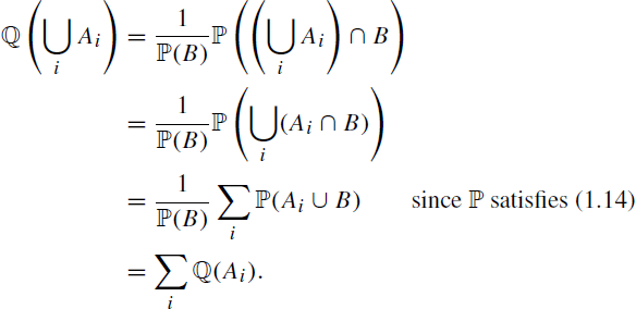
We speak of an event space as being ‘closed under the operations of taking complements and countable unions’. Here are some elementary consequences of axioms (1.2)–(1.4).

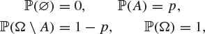
(a) An event space must contain the empty set and the whole set Ω. This holds as follows. By (1.2), there exists some . By (1.3), . We set , for in (1.4), and deduce that contains the union . By (1.3) again, the complement lies in also.

(b) An event space is closed under the operation of finite unions, as follows. Let , and set for . Then satisfies , so that by (1.4).

(c) The third condition (1.4) is written in terms of unions. An event space is also closed under the operations of taking finite or countable intersections. This follows by the elementary formula , and its extension to finite and countable families.

Here are some examples of pairs of sample spaces and event spaces.

Example 1.5

Ω is any non-empty set and is the power set of Ω.

Example 1.6

Ω is any non-empty set and , where A is a given non-trivial subset of Ω.

Example 1.7

and is the collection

of subsets of Ω. This event space is unlikely to arise naturally in practice.

In the following exercises, Ω is a set and is an event space of subsets of Ω.

Exercise 1.8

If , show that .

Exercise 1.9

The difference of two subsets A and B of Ω is the set of all points of Ω which are in A but not in B. Show that if , then .

Exercise 1.10

The symmetric difference of two subsets A and B of Ω is defined to be the set of points of Ω which are in either A or B but not both. If , show that .

Exercise 1.11

If and k is positive integer, show that the set of points in Ω which belong to exactly k of the A_i belongs to (the previous exercise is the case when and ).

Exercise 1.12

Show that, if Ω is a finite set, then contains an even number of subsets of Ω.

1.3 Probabilities

From our experiment , we have so far constructed a sample space Ω and an event space associated with , but there has been no mention yet of probabilities. The third thing which we do is to allocate probabilities to each event in , writing for the probability of the event A. We shall assume that this can be done in such a way that the probability function satisfies certain intuitively attractive conditions:

(a) each event A in the event space has a probability satisfying ,

(b) the event Ω, that ‘something happens’, has probability 1, and the event , that ‘nothing happens’, has probability 0,

We collect these conditions into a formal definition as follows.³

Definition 1.13

A mapping is called a probability measure on if

(a) for ,

(b) and ,

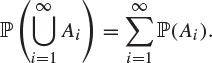
(1.14)

We emphasize that a probability measure on is defined only on those subsets of Ω which lie in . Here are two notes about probability measures.

(i) The second part of condition (b) is superfluous in the above definition. To see this, define the disjoint events , for . By condition (c),

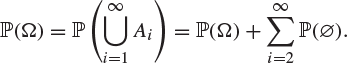
(ii) Condition (c) above is expressed as saying that is countably additive. The probability measure is also finitely additive in that

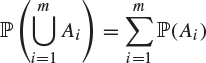
for disjoint events A_i. This is deduced from condition (c) by setting for .

Condition (1.14) requires that the probability of the union of a countable collection of disjoint sets is the sum of the individual probabilities.⁴

Example 1.15

Let Ω be a non-empty set and let A be a proper, non-empty subset of Ω (so that ). If is the event space , then all probability measures on have the form

for some p satisfying .

Example 1.16

Let be a finite set of exactly N points, and let be the power set of Ω. It is easy to check that the function defined by

is a probability measure on .⁵

Exercise 1.17

Let be non-negative numbers such that , and let , with the power set of Ω, as in Example 1.16. Show that the function given by

is a probability measure on . Is a probability measure on if is not the power set of Ω but merely some event space of subsets of Ω?

1.4 Probability spaces

We combine the previous ideas in a formal definition.

Definition 1.18

A probability space is a triple of objects such that

(a) Ω is a non-empty set,

(b) is an event space of subsets of Ω,

There are many elementary consequences of the axioms underlying this definition, and we describe some of these. Let be a probability space.

Property If , then⁶ .

Proof

The complement of equals , which is the union of events and is therefore an event. Hence is an event, by (1.3).

Property If , then .

Proof

The complement of equals , which is the union of the complements of events and is therefore an event. Hence the intersection of the A_i is an event also, as before.

Property If then .

Proof

The events A and are disjoint with union Ω, and so

Property If then .

Proof

The set A is the union of the disjoint sets and , and hence

A similar remark holds for the set B, giving that

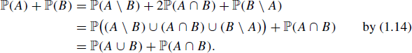
Property If and then .

Proof

We have that .

It is often useful to draw a Venn diagram when working with probabilities . For example, to illustrate the formula , we might draw the diagram in Figure 1.1, and note that the probability of is the sum of and minus , since the last probability is counted twice in the simple sum .

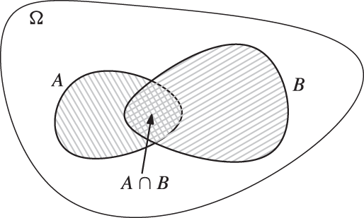
**Fig. 1.1** A Venn diagram illustrating the fact that .

In the following exercises, is a probability space.

Exercise 1.19

If , show that .

Exercise 1.20

If , show that

Exercise 1.21

Let be three events such that

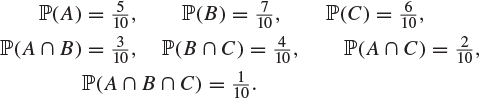
By drawing a Venn diagram or otherwise, find the probability that exactly two of the events A, B, C occur.

Exercise 1.22

A fair coin is tossed 10 times (so that heads appears with probability at each toss). Describe the appropriate probability space in detail for the two cases when

(a) the outcome of every toss is of interest,

(b) only the total number of tails is of interest.

In the first case your event space should have events, but in the second case it need have only events.

1.5 Discrete sample spaces

Let be an experiment with probability space . The structure of this space depends greatly on whether Ω is a countable set (that is, a finite or countably infinite set) or an uncountable set. If Ω is a countable set, we normally take to be the set of all subsets of Ω, for the following reason. Suppose that and, for each , we are interested in whether or not this given ω is the actual outcome of ; then we require that each singleton set belongs to . Let . Then A is countable (since Ω is countable), and so A may be expressed as the union of the countably many which belong to A, giving that by (1.4). The probability of the event A is determined by the collection of probabilities as ω ranges over Ω, since, by (1.14),

We usually write for the probability of an event containing only one point in Ω.

Example 1.23 (Equiprobable outcomes)

If and for all i and j, then for , and for .

Example 1.24 (Random integers)

There are ‘intuitively clear’ statements which are without meaning in probability theory, and here is an example: if we pick a positive integer at random, then it is an even integer with probability . Interpreting ‘at random’ to mean that each positive integer is equally likely to be picked, then this experiment would have probability space , where

(a) ,

(b) is the set of all subsets of Ω,

However,

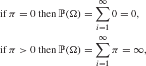
neither of which is in agreement with the rule that . One possible way of interpreting the italicized statement above is as follows. Let N be a large positive integer, and let be the experiment of picking an integer from the finite set at random. The probability that the outcome of is even is

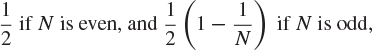
so that, as , the required probability tends to . Despite this sensible interpretation of the italicized statement, we emphasize that this statement is without meaning in its present form and should be shunned by serious probabilists.

The most elementary problems in probability theory are those which involve experiments such as the shuffling of cards or the throwing of dice, and these usually give rise to situations in which every possible outcome is equally likely to occur. This is the case of Example 1.23 above. Such problems usually reduce to the problem of counting the number of ways in which some event may occur, and the following exercises are of this type.

Exercise 1.25

Show that if a coin is tossed n times, then there are exactly

sequences of possible outcomes in which exactly k heads are obtained. If the coin is fair (so heads and tails are equally likely on each toss), show that the probability of getting at least k heads is

Exercise 1.26

We distribute r distinguishable balls into n cells at random, multiple occupancy being permitted. Show that

(a) there are possible arrangements,

(b) there are arrangements in which the first cell contains exactly k balls,

Exercise 1.27

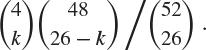
In a game of bridge, the 52 cards of a conventional pack are distributed at random between the four players in such a way that each player receives 13 cards. Show that the probability that each player receives one ace is

Exercise 1.28

Show that the probability that two given hands in bridge contain k aces between them is

Exercise 1.29

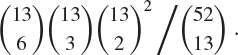
Show that the probability that a hand in bridge contains 6 spades, 3 hearts, 2 diamonds and 2 clubs is

Exercise 1.30

Which of the following is more probable:

(a) getting at least one six with 4 throws of a die,

(b) getting at least one double six with 24 throws of two dice?

This is sometimes called ‘de Méré’s paradox’, after the professional gambler Chevalier de Méré, who believed these two events to have equal probability.

1.6 Conditional probabilities

Let be an experiment with probability space . We may sometimes possess some incomplete information about the actual outcome of without knowing this outcome entirely. For example, if we throw a fair die and a friend tells us that an even number is showing, then this information affects our calculations of probabilities. In general, if A and B are events (that is, ) and we are given that B occurs, then, in the light of this information, the new probability of A may no longer be . Clearly, in this new circumstance, A occurs if and only if occurs, suggesting that the new probability of A should be proportional to . We make this chat more formal in a definition.⁷

Definition 1.31

If and , the (conditional) probability of A given B is denoted by and defined by

(1.32)

Note that the constant of proportionality in (1.32) has been chosen so that the probability , that B occurs given that B occurs, satisfies . We must next check that this definition gives rise to a probability space.

Theorem 1.33

If and then is a probability space where is defined by .

Proof

We need only check that is a probability measure on . Certainly for and

and it remains to check that satisfies (1.14). Suppose that are disjoint events in . Then

Exercise 1.34

If is a probability space and are events, show that

so long as .

Exercise 1.35

Show that

if and .

Exercise 1.36

Consider the experiment of tossing a fair coin 7 times. Find the probability of getting a prime number of heads given that heads occurs on at least 6 of the tosses.

1.7 Independent events

We call two events A and B ‘independent’ if the occurrence of one of them does not affect the probability that the other occurs. More formally, this requires that, if , , then

(1.37)

Writing , we see that the following definition is appropriate.

Definition 1.38

Events A and B of a probability space are called independent if

(1.39)

and dependent otherwise.

This definition is slightly more general than (1.37) since it allows the events A and B to have zero probability. It is easily generalized as follows to more than two events. A family of events is called independent if, for all finite subsets J of I,

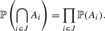
(1.40)

The family is called pairwise independent if (1.40) holds whenever .

Thus, three events, A, B, C, are independent if and only if the following equalities hold:

There are families of events which are pairwise independent but not independent.

Example 1.41

Suppose that we throw a fair four-sided die (you may think of this as a square die thrown in a two-dimensional universe). We may take , where each is equally likely to occur. The events , , are pairwise independent but not independent.

Exercise 1.42

Let A and B be events satisfying , , and such that . Show that .

Exercise 1.43

If A and B are events which are disjoint and independent, what can be said about the probabilities of A and B?

Exercise 1.44

Show that events A and B are independent if and only if A and are independent.

Exercise 1.45

Show that events are independent if and only if , are independent.

Exercise 1.46

If are independent and for , find the probability that

(a) none of the A_i occur,

(b) an even number of the A_i occur.

Exercise 1.47

On your desk, there is a very special die with a prime number p of faces, and you throw this die once. Show that no two events A and B can be independent unless either A or B is the whole sample space or the empty set.

1.8 The partition theorem

Let be a probability space. A partition of Ω is a collection of disjoint events (in that for each i, and if ) with union . The following partition theorem is extremely useful.

Theorem 1.48 (Partition theorem)

If is a partition of Ω with for each i, then

This theorem has several other fancy names such as ‘the theorem of total probability’, and it is closely related to ‘Bayes’ theorem’, Theorem 1.50.

Proof

We have that

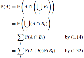
Here is an example of this theorem in action in a two-stage calculation.

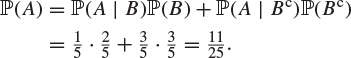
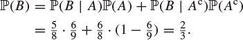
Example 1.49

Tomorrow there will be either rain or snow but not both; the probability of rain is and the probability of snow is . If it rains, the probability that I will be late for my lecture is , while the corresponding probability in the event of snow is . What is the probability that I will be late?

Solution

Let A be the event that I am late and B be the event that it rains. The pair B, is a partition of the sample space (since exactly one of them must occur). By Theorem 1.48,

There are many practical situations in which you wish to deduce something from a piece of evidence. We write A for the evidence, and for the possible ‘states of nature’. Suppose there are good estimates for the conditional probabilities , but we seek instead a probability of the form .

Theorem 1.50 (Bayes’ theorem)

Let be a partition of the sample space Ω such that for each i. For any event A with ,

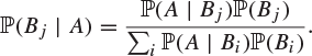
Proof

By the definition of conditional probability (see Exercise 1.35),

and the claim follows by the partition theorem, Theorem 1.48.

Example 1.51 (False positives)

A rare but potentially fatal disease has an incidence of 1 in in the population at large. There is a diagnostic test, but it is imperfect. If you have the disease, the test is positive with probability ; if you do not, the test is positive with probability . Your test result is positive. What is the probability that you have the disease?

Solution

Write D for the event that you have the disease, and P for the event that the test is positive. By Bayes’ theorem, Theorem 1.50,

It is more likely that the result of the test is incorrect than that you have the disease.

Exercise 1.52

Here are two routine problems about balls in urns. You are presented with two urns. Urn I contains 3 white and 4 black balls, and Urn II contains 2 white and 6 black balls.

(a) You pick a ball randomly from Urn I and place it in Urn II. Next you pick a ball randomly from Urn II. What is the probability that the ball is black?

(b) This time, you pick an urn at random, each of the two urns being picked with probability , and you pick a ball at random from the chosen urn. Given the ball is black, what is the probability you picked Urn I?

Exercise 1.53

A biased coin shows heads with probability whenever it is tossed. Let u_n be the probability that, in n tosses, no two heads occur successively. Show that, for ,

and find u_n by the usual method (described in Appendix B) when .

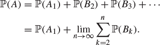
1.9 Probability measures are continuous

There is a certain property of probability measures which will be very useful later, and we describe this next. Too great an emphasis should not be placed on the property at this stage, and we recommend to the reader that he or she omit this section at the first reading.

A sequence of events in a probability space is called increasing if

The union

of such a sequence is called the limit of the sequence, and it is an elementary consequence of the axioms for an event space that A is an event. It is perhaps not surprising that the probability of A may be expressed as the limit of the probabilities of the A_n.

Theorem 1.54 (Continuity of probability measures)

Let be a probability space. If is an increasing sequence of events in with limit A, then

We precede the proof of the theorem with an application.

Example 1.55

It is intuitively clear that the chance of obtaining no heads in an infinite set of tosses of a fair coin is 0. A rigorous proof goes as follows. Let A_n be the event that the first n tosses of the coin yield at least one head. Then

so that the A_n form an increasing sequence. The limit set A is the event that heads occurs sooner or later. By the continuity of , Theorem 1.54,

However, , and so as . Thus , giving that the probability , that no head ever appears, equals 0.

Proof of Theorem 1.54

Let . Then

is the union of disjoint events in (draw a Venn diagram to make this clear). By (1.14),

However,

and so

as required, since the last sum collapses.

The conclusion of Theorem 1.54 is expressed in terms of an increasing sequence of events, but the corresponding statement for a decreasing sequence is valid too: if is a sequence of events in such that for , then as , where is the limit of the B_i as . The shortest way to show this is to set in the theorem.

1.10 Worked problems

Example 1.56

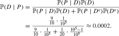
A fair six-sided die is thrown twice (when applied to such objects as dice or coins, the adjectives ‘fair’ and ‘unbiased’ imply that each possible outcome has equal probability of occurring).

(a) Write down the probability space of this experiment.

(b) Let B be the event that the first number thrown is no larger than 3, and let C be the event that the sum of the two numbers thrown equals 6. Find the probabilities of B and C, and the conditional probabilities of C given B, and of B given C.

Solution

The probability space of this experiment is the triple , where

(i) , the set of all ordered pairs of integers between 1 and 6,

(ii) is the set of all subsets of Ω,

(iii) each point in Ω has equal probability, so that

and, more generally,

The events B and C are subsets of Ω given by

The event B contains ordered pairs, and C contains 5 ordered pairs, giving that

Finally, is given by

containing just 3 ordered pairs, so that

and

Example 1.57

You are travelling on a train with your sister. Neither of you has a valid ticket, and the inspector has caught you both. He is authorized to administer a special punishment for this offence. He holds a box containing nine apparently identical chocolates, three of which are contaminated with a deadly poison. He makes each of you, in turn, choose and immediately eat a single chocolate.

(a) If you choose before your sister, what is the probability that you will survive?

(b) If you choose first and survive, what is the probability that your sister survives?

(d) Is it in your best interests to persuade your sister to choose first?

(e) If you choose first, what is the probability that you survive, given that your sister survives?

Solution

Let A be the event that the first chocolate picked is not poisoned, and let B be the event that the second chocolate picked is not poisoned. Elementary calculations, if you are allowed the time to perform them, would show that

giving by the partition theorem, Theorem 1.48, that

Hence , so that the only reward of choosing second is to increase your life expectancy by a few seconds.

The final question (e) seems to be the wrong way round in time, since your sister chooses her chocolate after you. The way to answer such a question is to reverse the conditioning as follows:

(1.58)

and hence

We note that , in agreement with our earlier observation that the order in which you and your sister pick from the box is irrelevant to your chances of survival.

Example 1.59

A coin is tossed times. What is the probability of exactly n heads? How does your answer behave for large n?

Solution

The sample space is the set of possible outcomes. It has elements, each of which is equally likely. There are ways to throw exactly n heads. Therefore, the answer is

(1.60)

To understand how this behaves for large n, we need to expand the binomial coefficient in terms of polynomials and exponentials. The relevant asymptotic formula is called Stirling’s formula,

(1.61)

where means as . See Theorem A.4 for a partial proof of this.

Applying Stirling’s formula to (1.60), we obtain

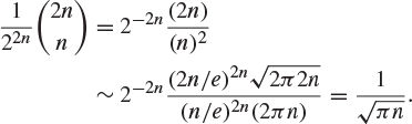
The factorials and exponentials are gigantic but they cancel out.

Example 1.62 (Simpson’s paradox)

The following comparison of surgical procedures is taken from Charig et al. (1986). Two treatments are considered for kidney stones, namely open surgery (abbreviated to OS) and percutaneous nephrolithotomy (PN). It is reported that OS has a success rate of () and PN a success rate of (). This looks like a marginal advantage to PN. On looking more closely, the patients are divided into two groups depending on whether or not their stones are smaller than 2 cm, with the following success rates.

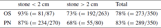
Open surgery wins in both cases! Discuss.

1.11 Problems

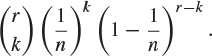
1. A fair die is thrown n times. Show that the probability that there are an even number of sixes is . For the purpose of this question, 0 is an even number.

2. Does there exist an event space containing just six events?

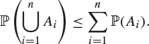
3. Prove Boole’s inequality:

4. Prove that

This is sometimes called Bonferroni’s inequality, but the term is not recommended since it has multiple uses.

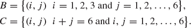
5. Two fair dice are thrown. Let A be the event that the first shows an odd number, B be the event that the second shows an even number, and C be the event that either both are odd or both are even. Show that A, B, C are pairwise independent but not independent.

6. Urn I contains 4 white and 3 black balls, and Urn II contains 3 white and 7 black balls. An urn is selected at random, and a ball is picked from it. What is the probability that this ball is black? If this ball is white, what is the probability that Urn I was selected?

7. A single card is removed at random from a deck of 52 cards. From the remainder we draw two cards at random and find that they are both spades. What is the probability that the first card removed was also a spade?

8. A fair coin is tossed times. Find the probability that the number of heads is twice the number of tails. Expand your answer using Stirling’s formula.

9. Two people toss a fair coin n times each. Show that the probability they throw equal numbers of heads is

10. In the circuits in Figure 1.2, each switch is closed with probability p, independently of all other switches. For each circuit, find the probability that a flow of current is possible between A and B.

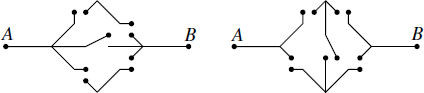
**Fig. 1.2** Two electrical circuits incorporating switches.

11. Show that if u_n is the probability that n tosses of a fair coin contain no run of 4 heads, then for

Use this difference equation to show that .

*12. Any number has a decimal expansion

and we write for the proportion of times that the integer k appears in the first n digits in this expansion. We call ω a normal number if

for . On intuitive grounds we may expect that most numbers are normal numbers, and Borel proved that this is indeed true. It is quite another matter to exhibit specific normal numbers. Prove the number

is normal. It is an unsolved problem of mathematics to show that and are normal numbers also.

13. A square board is divided into 16 equal squares by lines drawn parallel to its sides. A counter is placed at random on one of these squares and is then moved n times. At each of these moves, it can be transferred to any neighbouring square, horizontally, vertically, or diagonally, all such moves being equally likely.

Let c_n be the probability that a particular corner site is occupied after n such independent moves, and let the corresponding probabilities for an intermediate site at the side of the board and for a site in the middle of the board be s_n and m_n, respectively. Show that

and that

Find two other relations for s_n and m_n in terms of , , and , and hence find c_n, s_n, and m_n. (Oxford 1974M)

14. (a) Let denote the probability of the occurrence of an event A. Prove carefully, for events , that

(b) One evening, a bemused lodge-porter tried to hang n keys on their n hooks, but only managed to hang them independently and at random. There was no limit to the number of keys which could be hung on any hook. Otherwise, or by using (a), find an expression for the probability that at least one key was hung on its own hook.

The following morning, the porter was rebuked by the Bursar, so that in the evening she was careful to hang only one key on each hook. But she still only managed to hang them independently and at random. Find an expression for the probability that no key was then hung on its own hook.

Find the limits of both expressions as n tends to infinity.

You may assume that, for real x,

(Oxford 1978M)

15. Two identical decks of cards, each containing N cards, are shuffled randomly. We say that a k-matching occurs if the two decks agree in exactly k places. Show that the probability that there is a k-matching is

for . We note that for large N and fixed k. Such matching probabilities are used in testing departures from randomness in circumstances such as psychological tests and wine-tasting competitions. (The convention is that .)

16. The buses which stop at the end of my road do not keep to the timetable. They should run every quarter hour, at 08.30, 08.45, 09.00, . . . , but in fact each bus is either five minutes early or five minutes late, the two possibilities being equally probable and different buses being independent. Other people arrive at the stop in such a way that, t minutes after the departure of one bus, the probability that no one is waiting for the next one is . What is the probability that no one is waiting at 09.00? One day, I come to the stop at 09.00 and find no one there; show that the chances are more than four to one that I have missed the nine o’clock bus.

You may use an approximation . (Oxford 1977M)

17. A coin is tossed repeatedly; on each toss a head is shown with probability p, or a tail with probability . The outcomes of the tosses are independent. Let E denote the event that the first run of r successive heads occurs earlier that the first run of s successive tails. Let A denote the outcome of the first toss. Show that

Find a similar expression for , and hence find . (Oxford 1981M)

*18. Show that the axiom that is countably additive is equivalent to the axiom that is finitely additive and continuous. That is to say, let Ω be a set and an event space of subsets of Ω. If is a mapping from into satisfying

(i) ,

(ii) if and then ,

(iii) if and for then

where ,

then satisfies for all sequences of disjoint events.

19. There are n socks in a drawer, three of which are red and the rest black. John chooses his socks by selecting two at random from the drawer, and puts them on. He is three times more likely to wear socks of different colours than to wear matching red socks. Find n.

For this value of n, what is the probability that John wears matching black socks? (Cambridge 2008)