Probabilities

Did you believe me when I said few people probably passed along A Brief History of Time? I was using the term loosely, as many of us do, but the topic of mathematical probability confronts the very limits of what we can and cannot know about the world, stretching from the behavior of subatomic particles like quarks and bosons to the likelihood that the world will end in our lifetimes, from people playing a state lottery to trying to predict the weather (two endeavors that may have similar rates of success).

Probabilities allow us to quantify future events and are an important aid to rational decision making. Without them, we can become seduced by anecdotes and stories. You may have heard someone say something like “I’m not going to wear my seat belt because I heard about a guy who died in a car crash because he was wearing one. He got trapped in the car and couldn’t get out. If he hadn’t been wearing the seat belt, he would have been okay.”

Well, yes, but we can’t look at just one or two stories. What are the relative risks? Although there are a few odd cases where the seat belt cost someone’s life, you’re far more likely to die when not wearing one. Probability helps us look at this quantitatively.

We use the word probability in different ways to mean different things. It’s easy to get swept away thinking that a person means one thing when they mean another, and that confusion can cause us to draw the wrong conclusion.

One kind of probability—classic probability—is based on the idea of symmetry and equal likelihood: A die has six sides, a coin has two sides, a roulette wheel has thirty-eight slots (in the United States; thirty-seven slots in Europe). If there is no manufacturing defect or tampering that favors one outcome over another, each outcome is equally likely. So the probability of rolling any particular number on a die is one out of six, of getting heads on a coin toss is one out of two, of getting any particular slot on the roulette wheel is one out of thirty-seven or thirty-eight.

Classic probability is restricted to these kinds of well-defined objects. In the classic case, we know the parameters of the system and thus can calculate the probabilities for the events each system will generate. A second kind of probability arises because in daily life we often want to know something about the likelihood of other events occurring, such as the probability that a drug will work on a patient, or that consumers will prefer one beer to another. In this second case, we need to estimate the parameters of the system because we don’t know what those parameters are.

To determine this second kind of probability, we make observations or conduct experiments and count the number of times we get the outcome we want. These are called frequentist probabilities. We administer a drug to a group of patients and count how many people get better—that’s an experiment, and the probability of the drug working is simply the proportion of people for whom it worked (based on the frequency of the desired outcome). If we run the experiment on a large number of people, the results will be close to the true probability, just like public-opinion polling.

Both classic and frequentist probabilities deal with recurring, replicable events and the proportion of the time that you can expect to obtain a particular outcome under substantially the same conditions. (Some hard-liner probabilists contend they have to be identical conditions, but I think this takes it too far because in the limit, the universe is never exactly the same, due to chance variations.) When you conduct a public-opinion poll by interviewing people at random, you’re in effect asking them under identical conditions, even if you ask some today and some tomorrow—provided that some big event that might change their minds didn’t occur in between. When a court witness testifies about the probability of a suspect’s DNA matching the DNA found on a revolver, she is using frequentist probability, because she’s essentially counting the number of DNA fragments that match versus the number that don’t. Drawing a card from a deck, finding a defective widget on an assembly line, asking people if they like their brand of coffee are all examples of classic or frequentist probabilities that are recurring, replicable events (the card is classic, the widget and coffee are frequentist).

A third kind of probability differs from these first two because it’s not obtained from an experiment or a replicable event—rather, it expresses an opinion or degree of belief about how likely a particular event is to occur. This is called subjective probability (one type of this is Bayesian probability, after the eighteenth-century statistician Thomas Bayes). When a friend tells you that there’s a 50 percent chance that she’s going to attend Michael and Julie’s party this weekend, she’s using Bayesian probability, expressing a strength of belief that she’ll go. What will the unemployment rate be next year? We can’t use the frequentist method because we can’t consider next year’s unemployment as a set of observations taken under identical or even similar conditions.

Let’s think through an example. When a TV weather reporter says that there is a 30 percent chance of rain tomorrow, she didn’t conduct experiments on a bunch of identical days with identical conditions (if such a thing even exists) and then count the outcomes. The 30 percent number expresses her degree of belief (on a scale of one to a hundred) that it will rain, and is meant to inform you about whether you want to go to the trouble of grabbing your galoshes and umbrella.

If the weather reporter is well calibrated, it will rain on exactly 30 percent of the days for which she says there is a 30 percent chance of rain. If it rains on 60 percent of those days, she’s underestimated by a large amount. The issue of calibration is relevant only with subjective probabilities.

By the way, getting back to your friend who said there is a 50 percent chance she’ll attend a party, a mistake that many non–critical thinkers make is in assuming that if there are two possibilities, they must be equally likely. Cognitive psychologists Amos Tversky and Daniel Kahneman described parties and other scenarios to people in an experiment. At a particular party, for example, people might be told that 70 percent of the guests are writers and 30 percent are engineers. If you bump into someone with a tattoo of Shakespeare, you might correctly assume that person to be one of the writers; if you bump into someone wearing a Maxwell’s equations T-shirt, you might correctly assume that they are one of the engineers. But what if you bump into someone at random in the party and you’ve got nothing to go on—no Shakespeare tattoo, no math T-shirt—what’s the probability that this person is an engineer? In Tversky and Kahneman’s experiments, people tended to say, “Fifty-fifty,” apparently confusing the two possible outcomes with two equally likely outcomes.

Subjective probability is the only kind of probability that we have at our disposal in practical situations in which there is no experiment, no symmetry equation. When a judge instructs the jury to return a verdict if the “preponderance of evidence” points toward the defendant’s guilt, this is a subjective probability—each juror needs to decide for themselves whether a preponderance has been reached, weighing the evidence according to their own (and possibly idiosyncratic, not objective) internal standards and beliefs.

When a bookmaker lays odds for a horse race, he is using subjective probability—while it might be informed by data on the horses’ track records, health, and the jockeys’ history, there is no natural symmetry (meaning it’s not a classic probability) and there is no experiment being conducted (meaning it’s not a frequentist probability). The same is true for baseball and other sporting events. A bookie might say that the Royals have an 80 percent chance of winning their next game, but he’s not using probability in a mathematical sense; this is just a way he—and we—use language to give the patina of numerical precision. The bookie can’t turn back the hands of time and watch the Royals play the same game again and again, counting how many times they win it. He might well have crunched numbers or used a computer to inform his estimate, but at the end of the day, the number is just a guess, an indication of his degree of confidence in his prediction. A telltale piece of evidence that this is subjective is that different pundits come up with different answers.

Subjective probabilities are all around us and most of us don’t even realize it—we encounter them in newspapers, in the boardroom, and in sports bars. The probability that a rogue nation will set off an atomic bomb in the next twelve months, that interest rates will go up next year, that Italy will win the World Cup, or that soldiers will take a particular hill are all subjective, not frequentist: They are one-time, nonreplicable events. And the reputations of pundits and forecasters depend on their accuracy.

Combining Probabilities

One of the most important rules in probability is the multiplication rule. If two events are independent—that is, if the outcome of one does not influence the outcome of the other—you obtain the probability of both of them happening by multiplying the two probabilities together. The probability of getting heads on a coin toss is one half (because there are only two equally likely possibilities: heads and tails). The probability of getting a heart when drawing from a deck of cards is one-quarter (because there are only four equally likely possibilities: hearts, diamonds, clubs, and spades). If you toss a coin and draw a card, the probability of getting both heads and a heart is calculated by multiplying the two individual probabilities together: ½ × ¼ = ⅛. This is called a joint probability.

You can satisfy yourself that this is true by listing all possible cases and then counting how many times you get the desired outcome:

Head	Heart	Tail	Heart
Head	Diamond	Tail	Diamond
Head	Club	Tail	Club
Head	Spade	Tail	Spade

I’m ignoring the very rare occasions on which you toss the coin and it lands exactly on its side, or it gets carried off by a seagull while it’s in midair, or you have a trick deck of cards with all clubs.

We can similarly ask about the joint probability of three events: getting heads on a coin toss, drawing a heart from a deck of cards, and the next person you meet having the same birthday as you (the probability of that is roughly 1 out of 365.24—although births cluster a bit and some birthdates are more common than others, this is a reasonable approximation).

You may have visited websites where you are asked a series of multiple-choice questions, such as “Which of the following five streets have you lived on?” and “Which of the following five credit cards do you have?” These sites are trying to authenticate you, to be sure that you are who they think you are. They’re using the multiplication rule. If you answer six of these questions in a row, each with a probability of only one in five (.2) that you’ll get it right, the chances of you getting them right by simply guessing are only .2 × .2 × .2 × .2 × .2 × .2, or .000064—that’s about 6 chances in 100,000. Not as strict as what you find in DNA courtroom testimony, but not bad. (If you’re wondering why they don’t just ask you a bunch of short-answer, fill-in questions, where you have to provide the entire answer yourself, instead of using multiple choice, it’s because there are too many variants of correct answers. Do you refer to your credit card as being with Chase, Chase Bank, or JPMorgan Chase? Did you live on North Sycamore Street, N. Sycamore Street, or N. Sycamore St.? You get the idea.)

When the Probability of Events Is Informed by Other Events

The multiplication rule only applies if the events are independent of one another. What events are not independent? The weather, for example. The probability of it freezing tonight and freezing tomorrow night are not independent events—weather patterns tend to remain for more than one day, and although freak freezes are known to occur, your best bet about tomorrow’s overnight temperatures is to look at today’s. You could calculate the number of nights in the year in which temperatures drop below freezing—let’s say it’s thirty-six where you live—and then state that the probability of a freeze tonight is 36 out of 365, or roughly 10 percent, but that doesn’t take the dependencies into account. If you say that the probability of it freezing two nights in a row during winter is 10% × 10% = 1% (following the multiplication rule), you’d be underestimating the probability because the two nights’ events are not independent; tomorrow’s weather forecast is informed by today’s.

The probability of an event can also be informed by the particular sample that you’re looking at. The probability of it freezing tonight is obviously affected by the area of the world you’re talking about. That probability is higher at the forty-fourth parallel than the tenth. The probability of finding someone over six foot six is greater if you’re looking at a basketball practice than at a tavern frequented by jockeys. The subgroup of people or things you’re looking at is relevant to your probability estimate.

Conditional Probabilities

Often when looking at statistical claims, we’re led astray by examining an entire group of random people when we really should be looking at a subgroup. What is the probability that you have pneumonia? Not very high. But if we know more about you and your particular case, the probability may be higher or lower. This is known as a conditional probability.

We frame two different questions:

1. What is the probability that a person drawn at random from the population has pneumonia?
2. What is the probability that a person not drawn at random, but one who is exhibiting three symptoms (fever, muscle pain, chest congestion) has pneumonia?

The second question involves a conditional probability. It’s called that because we’re not looking at every possible condition, only those people who match the condition specified. Without running through the numbers, we can guess that the probability of pneumonia is greater in the second case. Of course, we can frame the question so that the probability of having pneumonia is lower than for a person drawn at random:

1. What is the probability that a person not drawn at random, but one who has just tested negative for pneumonia three times in a row, and who has an especially robust immune system, and has just minutes ago finished first place in the New York City Marathon, has pneumonia?

Along the same lines, the probability of you developing lung cancer is not independent of your family history. The probability of a waiter bringing ketchup to your table is not independent of what you ordered. You can calculate the probability of any person selected at random developing lung cancer in the next ten years, or the probability of a waiter bringing ketchup to a table calculated over all tables. But we’re in the lucky position of knowing that these events are dependent on other behaviors. This allows us to narrow the population we’re studying in order to obtain a more accurate estimate. For example, if your father and mother both had lung cancer, you want to calculate the probability of you contracting lung cancer by looking at other people in this select group, people whose parents had lung cancer. If your parents didn’t have lung cancer, you want to look at the relevant subgroup of people who lack a family history of it (and you’ll likely come up with a different figure). If you want to know the probability that your waiter will bring you ketchup, you might look at only the tables of those patrons who ordered hamburgers or fries, not those who ordered tuna tartare or apple pie.

Ignoring the dependence of events (assuming independence) can have serious consequences in the legal world. One was the case of Sally Clark, a woman from Essex, U.K., who stood trial for murdering her second child. Her first child had died in infancy, and his death had been attributed to SIDS (sudden infant death syndrome, or crib death). The prosecutors argued that the odds of having two children die of SIDS were so low that she must have murdered the second child. The prosecution’s witness, a pediatrician, cited a study that said SIDS occurred in 1 out of 8,543 infant deaths. (Dr. Meadow’s expertise in pediatrics does not make him an expert statistician or epidemiologist—this sort of confusion is the basis for many faulty judgments and is discussed in Part 3 of this book; an expert in one domain is not automatically an expert in another, seemingly related, domain.)

Digging deeper, we might question the figure of 8,543 deaths. How do they know that? SIDS is a diagnosis of exclusion—that is, there is no test that medical personnel can perform to conclude a death was by SIDS. Rather, if doctors are not able to find the cause, and they’ve ruled out everything else, they label it SIDS. Not being able to find something is not proof that it didn’t occur, so it is plausible that some of the deaths attributed to SIDS were actually the result of less mysterious causes, such as poisoning, suffocation, heart defect, etc.

For the sake of argument, however, let’s assume that SIDS is the cause of 1 out of 8,543 infant deaths as the expert witness testified. He further testified that the odds of two SIDS deaths occurring in the same family were ¹⁄₈₅₄₃ × ¹⁄₈₅₄₃, or 1 in 73 million. (“Coincidence? I think not!” the prosecutor might have shouted during his summation.) This calculation—this application of the multiplication rule—assumes the deaths are independent, but they might not be. Whatever caused Mrs. Clark’s first child to die suddenly might be present for both children by virtue of them being in the same household: Two environmental factors associated with SIDS are secondhand smoke and putting a baby to sleep on its stomach. Or perhaps the first child suffered from a congenital defect of some sort; this would have a relatively high probability of appearing in the second child’s genome (siblings share 50 percent of their DNA). By this way of thinking, there was a 50 percent chance that the second child would die due to a factor such as this, and so now Mrs. Clark looks a lot less like a child murderer. Eventually, her husband found evidence in the hospital archives that the second child’s death had a microbiological cause. Mrs. Clark was acquitted, but only after serving three years in prison for a crime she didn’t commit.

There’s a special notation for conditional probabilities. The probability of a waiter bringing you ketchup, given that you just ordered a hamburger, is written:

P(ketchup | hamburger)

where the vertical bar | is read as given. Note that this notation leaves out a lot of the words from the English-language description, so that the mathematical expression is succinct.

The probability of a waiter bringing you ketchup, given that you just ordered a hamburger and you asked for the ketchup, is noted:

P(ketchup | hamburger ∧ asked)

where the ∧ is read as and.

Visualizing Conditional Probabilities

The relative incidence of pneumonia in the United States in one year is around 2 percent—six million people out of the 324 million in the country are diagnosed each year (of course there are no doubt many undiagnosed cases, as well as individuals who may have more than one case in a year, but let’s ignore these details for now). Therefore the probability of any person drawn at random having pneumonia is approximately 2 percent. But we can home in on a better estimate if we know something about that particular person. If you show up at the doctor’s office with coughing, congestion, and a fever, you’re no longer a person drawn at random—you’re someone in a doctor’s office showing these symptoms. You can methodically update your belief that something is true (that you have pneumonia) in light of new evidence. We do this by applying Bayes’s rule to calculate a conditional probability: What is the probability that I have pneumonia given that I show symptom x? This kind of updating can become increasingly refined the more information you have. What is the probability that I have pneumonia given that I have these symptoms, and given that I have a family history of it, and given that I just spent three days with someone who has it? The probabilities climb higher and higher.

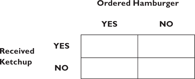
You can calculate the probabilities using the formula for Bayes’s rule (found in the Appendix), but an easy way to visualize and compute conditional probabilities is with the fourfold table, describing all possible scenarios: You did or didn’t order a hamburger, and you did or didn’t receive ketchup:

Then, based on experiments and observation, you fill in the various values, that is, the frequencies of each event. Out of sixteen customers you observed at a restaurant, there was one instance of someone ordering a hamburger with which they received ketchup, and two instances with which they didn’t. These become entries in the left-hand column of the table:

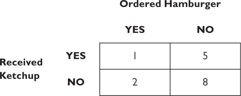
Similarly, you found that five people who didn’t order a hamburger received ketchup, and eight people did not. These are the entries in the right-hand column.

Next, you sum the rows and columns:

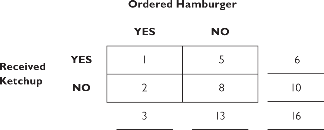
Now, calculating the probabilities is easy. If you want to know the probability that you received ketchup given that you ordered a hamburger, you start with the given. That’s the left-hand vertical column.

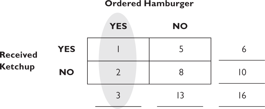
Three people ordered hamburgers altogether—that’s the total at the bottom of the column. Now what is the probability of receiving ketchup given you ordered a hamburger? We look now at the “YES received ketchup” square in the “YES ordered hamburger” column, and that number is 1. The conditional probability, P(ketchup|hamburger) is then just one out of three. And you can visualize the logic: three people ordered a hamburger; one of them got ketchup and two didn’t. We ignore the right-hand column for this calculation.

We can use this to calculate any conditional probability, including the probability of receiving ketchup if you didn’t order a hamburger: Thirteen people didn’t order a hamburger, five of them got ketchup, so the probability is five out of thirteen, or about 38 percent. In this particular restaurant, you’re more likely to get ketchup if you didn’t order a hamburger than if you did. (Now fire up your critical thinking. How could this be? Maybe the data are driven by people who ordered fries. Maybe all the hamburgers served already have ketchup on them.)

Medical Decision Making

This way of visualizing conditional probabilities is useful for medical decision making. If you take a medical test, and it says you have some disease, what is the probability you actually have the disease? It’s not 100 percent, because the tests are not perfect—they produce false positives (reporting that you have the disease when you don’t) and false negatives (reporting that you don’t have the disease when you do).

The probability that a woman has breast cancer is 0.8 percent. If she has breast cancer, the probability that a mammogram will indicate it is only 90 percent because the test isn’t perfect and it misses some cases. If the woman does not have breast cancer, the probability of a positive result is 7 percent. Now, suppose a woman, drawn at random, has a positive result—what is the probability that she actually has breast cancer?

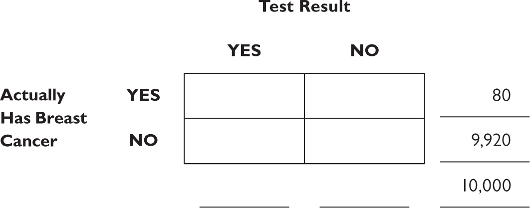
We start by drawing a fourfold table and filling in the possibilities: The woman actually has breast cancer or doesn’t, and the test can report that she does or that she doesn’t. To make the numbers work out easily—to make sure we’re dealing with whole numbers—let’s assume we’re talking about 10,000 women.

That’s the total population, and so that number goes in the lower right-hand corner of the figure, outside the boxes.

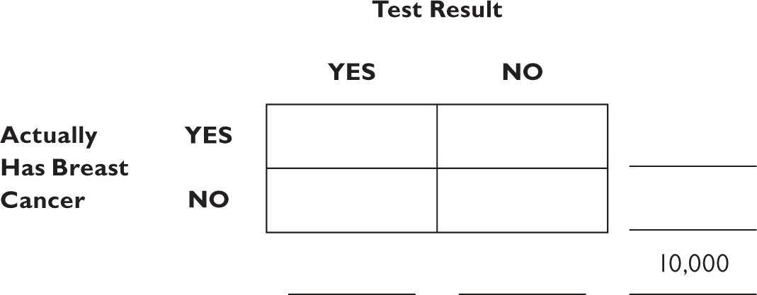
Unlike the hamburger-ketchup example, we fill in the margins first, because that’s the information we were given. The probability of breast cancer is 0.8 percent, or 80 out of 10,000 people. That number goes in the margin of the top row. (We don’t yet know how to fill in the boxes, but we will in a second.) And because the row has to add up to 10,000, we know that the margin for the bottom row has to equal

10,000 − 80 = 9,920.

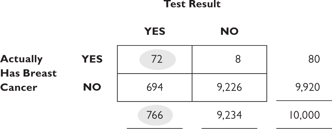
We were told that the probability that the test will show a positive if breast cancer exists is 90 percent. Because probabilities have to add up to 100 percent, the probability that the test will not show a positive result if breast cancer exists has to be 100 percent − 90 percent, or 10 percent. For the eighty women who actually have breast cancer (the margin for the top row), we now know that 90 percent of them will have a positive test result (90% of 80 = 72) and 10 percent will have a negative result (10% of 80 = 8). This is all we need to know how to fill in the boxes on the top row.

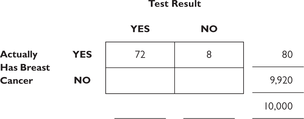
We’re not yet ready to calculate the answer to questions such as “What is the probability that I have breast cancer given that I had a positive test result?” because we need to know how many people will have a positive test result. The missing piece of the puzzle is in the original description: 7 percent of women who don’t have breast cancer will still show a positive result. The margin for the lower row tells us 9,920 women don’t have breast cancer; 7 percent of them = 694.4. (We’ll round to 694.) That means that 9,920 − 694 = 9,226 goes in the lower right square.

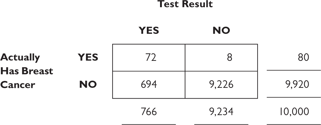
Finally, we add up the columns.

If you’re among the millions of people who think that having a positive test result means you definitely have the disease, you’re wrong. The conditional probability of having breast cancer given a positive test result is the upper left square divided by the left column’s margin total, or ⁷²⁄₇₆₆. The good news is that, even with a positive mammogram, the probability of actually having breast cancer is 9.4 percent. This is because the disease is relatively rare (less than 1 in 1,000) and the test for it is imperfect.

Conditional Probabilities Do Not Work Backward

We’re used to certain symmetries in math from grade school: If x = y then y = x. 5 + 7 = 7 + 5. But some concepts don’t work that way, as we saw in the discussion above on probability values (if the probability of a false alarm is 10 percent, that doesn’t mean that the probability of a hit is 90 percent).

Consider the statistic:

Ten times as many apples are sold in supermarkets as in roadside stands.

A little reflection should make it apparent that this does not mean you’re more likely to find an apple on the day you want one by going to the supermarket: The supermarket may have more than ten times the number of customers as roadside stands have, but even with its greater inventory, it may not keep up with demand. If you see a random person walking down the street with an apple, and you have no information about where they bought it, the probability is higher that they bought it at a supermarket than at a roadside stand. We can ask, as a conditional probability, what is the probability that this person bought it at a supermarket given that they have an apple?

P(was in a supermarket | found an apple to buy)

It is not the same as what you might want to know if you’re craving a Honeycrisp:

P(found an apple to buy | was in a supermarket)

This same asymmetry pops up in various disguises, in all manner of statistics. If you read that more automobile accidents occur at seven p.m. than at seven a.m., what does that mean? Here, the language of the statement itself is ambiguous. It could either mean you’re looking at the probability that it was seven p.m. given that an accident occurred, or the probability that an accident occurred given that it was seven p.m. In the first case, you’re looking at all accidents and seeing how many were at seven p.m. In the second case, you’re looking at how many cars are on the road at seven p.m., and seeing what proportion of them are involved in accidents. What?

Perhaps there are far more cars on the road at seven p.m. than any other time of day, and far fewer accidents per thousand cars. That would yield more accidents at seven p.m. than any other time, simply due to the larger number of vehicles on the road. It is the accident rate that helps you determine the safest time to drive.

Similarly, you may have heard that most accidents occur within three miles of home. This isn’t because that area is more dangerous per se, it’s because the majority of trips people take are short ones, and so the three miles around the home is much more traveled. In most cases, these two different interpretations of the statement will not be equivalent:

P(7 p.m. | accident) ≠ P(accident | 7 p.m.)

The consequences of such confusion are hardly just theoretical: Many court cases have hinged on a misapplication of conditional probabilities, confusing the direction of what is known. A forensics expert may compute, correctly, that the probability of the blood found at the crime scene matching the defendant’s blood type by chance is only 1 percent. This is not at all the same as saying that there is only a 1 percent chance the defendant is innocent. What? Intuition tricks us again. The forensics expert is telling us the probability of a blood match given that the defendant is innocent:

P(blood match | innocence)

Or, in plain language, “the probability that we would find a match if the defendant were actually innocent.” That is not the same as the number you really want to know: What is the probability that the defendant is innocent given that the blood matched:

P(blood match | innocence) ≠ P(innocence | blood match)

Many innocent citizens have been sent to prison because of this misunderstanding. And many patients have made poor decisions about medical care because they thought, mistakenly, that

P(positive test result | cancer) = P(cancer | positive test result)

And it’s not just patients—doctors make this error all the time (in one study 90 percent of doctors treated the two different probabilities the same). The results can be horrible. One surgeon persuaded ninety women to have their healthy breasts removed if they were in a high-risk group. He had noted that 93 percent of breast cancers occurred in women who were in this high-risk group. Given that a woman had breast cancer, there was a 93 percent chance she was in this group: P(high-risk group | breast cancer) = .93. Using a fourfold table for a sample of 1,000 typical women, and adding the additional information that 57 percent of women fall into this high-risk group, and that the probability of a woman having breast cancer is 0.8 percent (as mentioned earlier), we can calculate P(breast cancer | high-risk group), which is the statistic a woman needs to know before consenting to the surgery (numbers are rounded to the nearest integer):

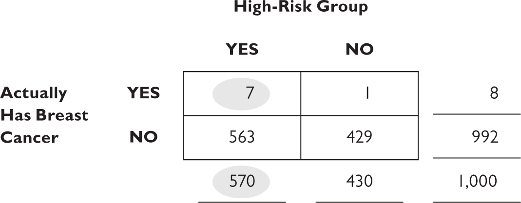
The probability that a woman has cancer, given that she is in this high-risk group is not 93 percent, as the surgeon erroneously thought, but only ⁷⁄₅₇₀, or 1 percent. The surgeon overestimated the cancer risk by nearly one hundred times the actual risk. And the consequences were devastating.

The fourfold tables might feel like a strange little exercise, but actually what you’re doing here is scientific and critical thinking, laying out the numbers visually in order to make the computation easier. And the results of those computations allow you to quantify the different parts of the problem, to help you make more rational, evidence-based decisions. They are so powerful, it’s surprising that they’re not taught to all of us in high school.

Thinking About Statistics and Graphs

Most of us have difficulty figuring probabilities and statistics in our heads and detecting subtle patterns in complex tables of numbers. We prefer vivid pictures, images, and stories. When making decisions, we tend to overweight such images and stories, compared to statistical information. We also tend to misunderstand or misinterpret graphics.

Many of us feel intimidated by numbers and so we blindly accept the numbers we’re handed. This can lead to bad decisions and faulty conclusions. We also have a tendency to apply critical thinking only to things we disagree with. In the current information age, pseudo-facts masquerade as facts, misinformation can be indistinguishable from true information, and numbers are often at the heart of any important claim or decision. Bad statistics are everywhere. As sociologist Joel Best says, it’s not just because the other guys are all lying weasels. Bad statistics are produced by people—often sincere, well-meaning people—who aren’t thinking critically about what they’re saying.

The same fear of numbers that prevents many people from analyzing statistics prevents them from looking carefully at the numbers in a graph, the axis labels, and the story that they tell. The world is full of coincidences and bizarre things are very likely to happen—but just because two things change together doesn’t mean that one caused the other or that they are even related by a hidden third factor x. People who are taken in by such associations or coincidences usually have a poor understanding of probability, cause and effect, and the role of randomness in the unfolding of events. Yes, you could spin a story about how the drop in the number of pirates over the last three hundred years and the coinciding rise in global temperatures must surely indicate that pirates were essential to keeping global warming under control. But that’s just sloppy thinking, and is a misinterpretation of the evidence. Sometimes the purveyors of this sort of faulty logic know better and hope that you won’t notice; sometimes they have been taken in themselves. But now you know better.